Contents

In this post, we’ll go through:

(i) Role of Support Vectors in SVMs

(ii) Cost Function for SVMs

(iii) SVMs as a Large Margin Classifier

(iv) Non-Linear Decision Boundaries through SVMs with the help of Kernels

(v) Fraudulent Credit Card Transaction Kaggle Dataset Detection using SVMs

In the previous post, we had a good look at high bias and variance problems in machine learning and discussed how regularization plays a big role in solving these issues along with some other techniques. In this post, we’ll be having a detailed look at another supervised learning algorithm called the Support Vector Machine. Later in the post, we’ll be solving a Kaggle dataset to detect Fraudulent Credit Card Transactions using the SVM.

Support Vector Machines (SVM)

SVM is a supervised machine learning method which solves both, regression and classification problems. However, it is mostly used in classification problems where it constructs hyperplanes in the n-feature dimensions. An n-dimension feature space has a hyperplane of n-1 dimensions. Eg. In the dataset with 2 features (2-dimeansional feature space), the hyperplane constructed by the SVM is a curve(line, circle, etc.) If we are solving a classification problem on 2 classes, then the job of the SVM classifier is to find the hyperplane that maximizes the margin between the 2 classes. Before we look at how SVMs work, let’s understand where the name Support Vector Machine came from.

SVM in action (Source)

What is a Support Vector?

We know that an SVM classifier constructs hyperplanes for classification. But how does the SVM classifier construct a hyperplane? Let’s develop intuition by considering just 2 classes. We know that a hyperplane has to pass from somewhere in the middle of the 2 classes. A good separation between these classes is achieved by the hyperplane that has the largest distance to the nearest training data points from both the classes. In the figure above, the 2 dotted lines that mark the extremes of each class constitute the support vectors for each class. These support vectors help in finding the hyperplane that maximizes the distance (margin) of the hyperplane from each of the 2 classes with the help of their support vectors.

Working of SVMs

Support Vector Machines can fit both linear and non-linear decision boundaries as a classifier and one of the main advantages SVMs have over Logistic Regression is that they compute the training parameters fast due to a much simplified cost function.

Cost Function

Let’s recall the binary crossentropy cost function used for binary classification in logistic regression. Here, for the sake of simplification, we’ll ignore the bias term, so the final prediction that we make for the ith training example out of a total of ‘m’ training examples through logistic regression will be represented as h(x(i)) = sigmoid(W * x(i))

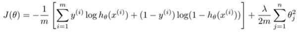
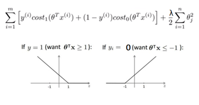
This cost function can be divided into 2 parts: when y(i) = 1 the term (1 — y(i))*log(1 — h(x(i))) becomes 0 and when y(i) = 0, the term y(i)*log(h(x(i))) becomes 0. The corresponding graphs for these equations (Cost vs W * x) (excluding the regularization term, since it is common to both) are:

SVM uses a slight modification of this cost function which provides it computational advantages over logistic regression. For the case y = 1, we see that the cost function has all its values closer to 0 when W * x >= 1 and when W * x < 1, the -log(h(x)) function values are approximated by a straight line by calculating the derivative of the cost function when W * x = 0. Similarly for the case y = 0, we see that the cost function has all its values closer to 0 when W * x <= -1 and when W * x > 1, the -log(1 — h(x)) values are approximated by a straight line by calculating the derivative of the cost function when W * x = 0.

Now since we are no longer using logarithmic cost function, let’s rename the log part in the logistic regression cost function. Let’s replace **-log(h(x)) with cost1(h(x)) **and -log(1 — h(x)) with cost0(h(x)). We’re ignoring the constant (1/m) here as it doesn’t affect our minimization objective and helps us to simplify our calculations. So, the final cost function for support vector machine looks like:

This leads to the following mathematical equation for the cost function:

Unlike logistic regression which outputs probability values, SVMs output 0/1. When h(x) >=1, the SVM outputs 1 and when h(x) <= -1, the SVM outputs 0. In logistic regression, we saw that when h(x) > 0, the output was a probability > 0.5, which was rounded-off to 1 and when h(x) < 0, the output was a probability < 0.5 which was rounded-off to 0. The range of (-1, 1) is an _extra safety margin factor _which allows SVMs to make more confident predictions than logistic regression.

Let us now re-parameterize the cost function a bit. Currently our cost function is of the form A + λB, where A is the cost function and B is the regularization term. Let’s convert it to CA + B form, where C plays a role similar to 1/λ.

#machine-learning #python #kernel #support-vector-machine #kaggle