R for Data Analytics: A Beginners Guide

If you are thinking of getting into R, this article will give you a starting point. Through this article, I have tried to give a basic insight into data analytics using R.

Installing R and R studio

You can download the setup file for R from “here”. Once this is sorted, you will need an IDE to start programming in R. RStudio will do just fine for an IDE and you can download a free desktop version from “here”. After downloading and installing the aforementioned software, you are all set to begin your programming journey with R. Now, you may open R Studio, click on File, New File, and lastly on R Script.

Let’s begin Data analytics with R.

Installing Packages and Importing Libraries

You need not reinvent the wheel every time you build a car. So is true for programming as well. A library is a collection of functions that are developed to perform certain tasks. So each time a programmer writes a code, instead of writing tens and hundreds of lines just to perform a simple operation such as finding a square root, he/she and directly use the readily available function in the default library of R. Packages are a collection of libraries.

Since the purpose of this article is just to familiarize with the basics of the R, we will be generally focusing on data wrangling and data visualization aspect of data analytics. I will cover modeling and other high-level concepts in the follow-up articles.

For data wrangling we will be using the following libraries:

dplyr: The go-to package for data wrangling. used for manipulating rows and columns of data sets and even joining separate data sets together.
tidyr: Pretty much as the name suggests, used for tidying the data.
lubridate: Used to manipulate and re-format dates and time.
**forcats: **Used to handle categorical variables. More on this in the follow-ups.

For data visualization, **ggplot2 **has pretty much everything you will be needing.

The list of useful libraries goes long, however, don’t fret too much about memorizing the name of every library required for effectively. For this purpose, we have packages like “tidyverse”. This package has got all the aforementioned libraries and many more. So let’s install this package to R and import it to our program with the below lines of instruction:

#Installs package
install.packages(“tidyverse”) 

#Load core tidyverse package
library(tidyverse)

Importing the Data set

For analysis, we will be using a data set of 1000 most popular based on IMDB reviews. The data has been collected from “Kaggle” and has been compiled by the data creator promptcloud. The data set was last updated in June 2017 therefore, the accuracy in today’s scenario cannot be ascertained. However, we are using this data set for demonstration purposes only so it will serve just fine for our purpose. After downloading the data set from the above link and placing it in a directory of our choice, now we are ready to import the data to our R script.

mydata = read.csv("<path>") #Replace <path> with the path of file

If you have stored your file in the working directory, you can directly call out the file name. But before that, you will have to set up the folder where you have saved the file as a working directory. Post which you can directly call out the file name.

setwd("<path>")

#Data set will be stored in mydata data frame
mydata = read.csv("IMDB_moviedata.csv")

In my case, the file is stored as “IMDB_moviedata.csv”. CSV means comma-separated values. In this format, each element of data is separated by a comma. Although other characters can also be used to separate the elements of the data. To get more detail you can go through the R documentation by using the following command:

help(read.csv) #or
?read.csv

Tidying up the data

Now we have our data set imported, but in most cases, we cannot use it directly as it may not be correctly ordered or it might contain some features which are not required for our analysis. Before doing that, let’s first have a look at our data. You can use all or any of the below listed commands to do so.

head(mydata) #or
summary(mydata) #or
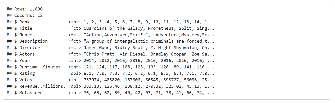
glimpse(mydata)

Below is a snippet of results from the glimpse function.

Image for post

So let’s begin tidying up the data.

#removing Description column
mydata <- select(mydata, -Description) 

#Assign NA to all blank entries
mydata <- mydata %>% mutate_all(na_if,"")
#Remove rows with NAs and store as mydata_cleaned
mydata_cleaned <- na.omit(mydata)
#Renaming the columns
mydata_cleaned %>% rename(Runtime_mins = Runtime..Minutes., Revenue_mills = Revenue..Millions.) -> mydata_cleaned
#Get the summary of clean data
summary(mydata_cleaned)

Data Visualization and Analysis

In this section, we will be performing some basic analysis of the imported data set. At first, let us compare the earnings of the top 10 rated movies. In our data set the movies have already been arranged as per their ranks. We will start by picking the top 10 movies from the data frame and comparing the revenue earned by them.

#selecting top 10 movies
top_ten <- head(mydata_cleaned, 10)

#subsetting revenue variable
var1 <- c("Rank", "Title", "Revenue_mills")
revenue_data <- top_ten[var1]
#viewing subsetted data frame
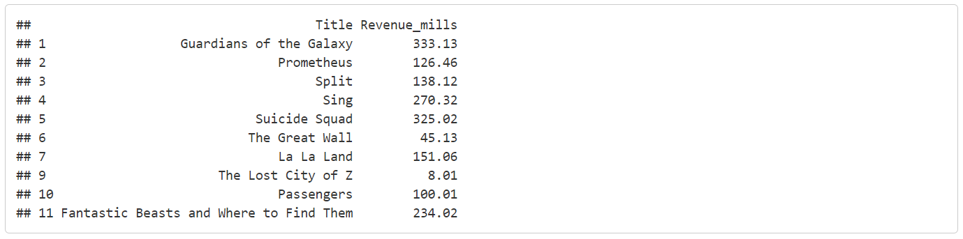
head(revenue_data)

Below is the data frame that we will be using to carry out this piece of analysis. Note that Rank 8 is missing. This is because rows with missing values were removed during the data cleaning process.