Random Forest & Gradient Boosting Algorithms

Tip It’s recommended that you should read the following articles regarding “Decision Tree: Regression Trees” and ”Decision Trees Classifier” before going deep in ensemble methods.

Introduction

The basic idea behind ensemble methods is to build a group or ensemble of different predictive models -weak models- (each of these models is independent of the others) and then combine their outputs in some way to get a precise final predicted value.

As using different algorithms to train different models (independent models) and combining their results is very very difficult, ensemble methods uses only one algorithm to train all of these models in a way to be completely independent.

So, ensemble methods employ a hierarchy of two algorithms.

1. The low-level algorithm is called a _base learner_. The base learner is a single machine learning algorithm that gets used for all of the models that will get aggregated into an ensemble.
2. The upper-level algorithm (e.g. Bagging, random forest and gradient boosting algorithms) manipulates the inputs to the base learners so that the models they generate are somewhat independent.

Many algorithms could be used as base-learner such as linear regression, SVM, but the in practical, binary decision-trees algorithm was chosen to be the default base learner of the ensemble methods.

The ensembles may consists of a contribution of hundreds or may thousands of binary decision trees, and of course inherit their properties from it.

Random Forest

There are two ensemble learning paradigms: bagging (abbreviation of bootstrap aggregation) and boosting. The bagging paradigm is behind the random forest algorithm whereas boosting paradigm is behind gradient boosting algorithm.

How Does the Bagging Algorithm Work?

• The bootstrap aggregation algorithm uses what is called a bootstrap sample.
• Bootstrap sample represents a group of data that being selected randomly from the original data set with replacement.
• Replacement means that, a bootstrap sample may contain multiple copies of a certain row/observation from the original data as the selection from original data set being done randomly one by one and that’s Ok.
• Each sample contains a number of instances of about 60% of the nubmer of instances within the original data set (with replacement).
• The job of bootstrap aggregation algorithm is to train each base learner with one of these samples.
• The resulting models are averaged in regression problems.

Where: _𝑦_̂ : is the average predicted output and _𝑆 _: is number of samples.

• For classification problems, the models can either be averaged or probabilities can be developed based on the percentages of different classes.
• Sufficient depth for decision trees will lead to a proper work and more precise predictions for bagging algorithm
• Random forest is so called parallel model.

Fig.1 Bagging Algorithm

Different from Bagging

The random forest algorithm has an advantage over bagging algorithm that, the training samples don’t incorporate all the attributes (columns) of the original data set, instead they take a random subset of them also.

Advantages

Random forest is one of the most widely used ensemble learning algorithms. Why is it so effective? The reason is that by using multiple samples of the original dataset, we reduce the variance of the final model. Remember that the low variance means low overfitting. Overfitting happens when our model tries to explain small variations in the dataset because our dataset is just a small sample of the population of all possible examples of the phenomenon we try to model.

Gradient Boosting

Gradient boosting develops an ensemble of tree-based models by training each of the trees in the ensemble on different labels and then combining the trees.

For a regression problem

Where the objective is to minimize residuals (errors), each successive tree is trained on the errors left over by the collection of earlier trees. Let’s see how it works?

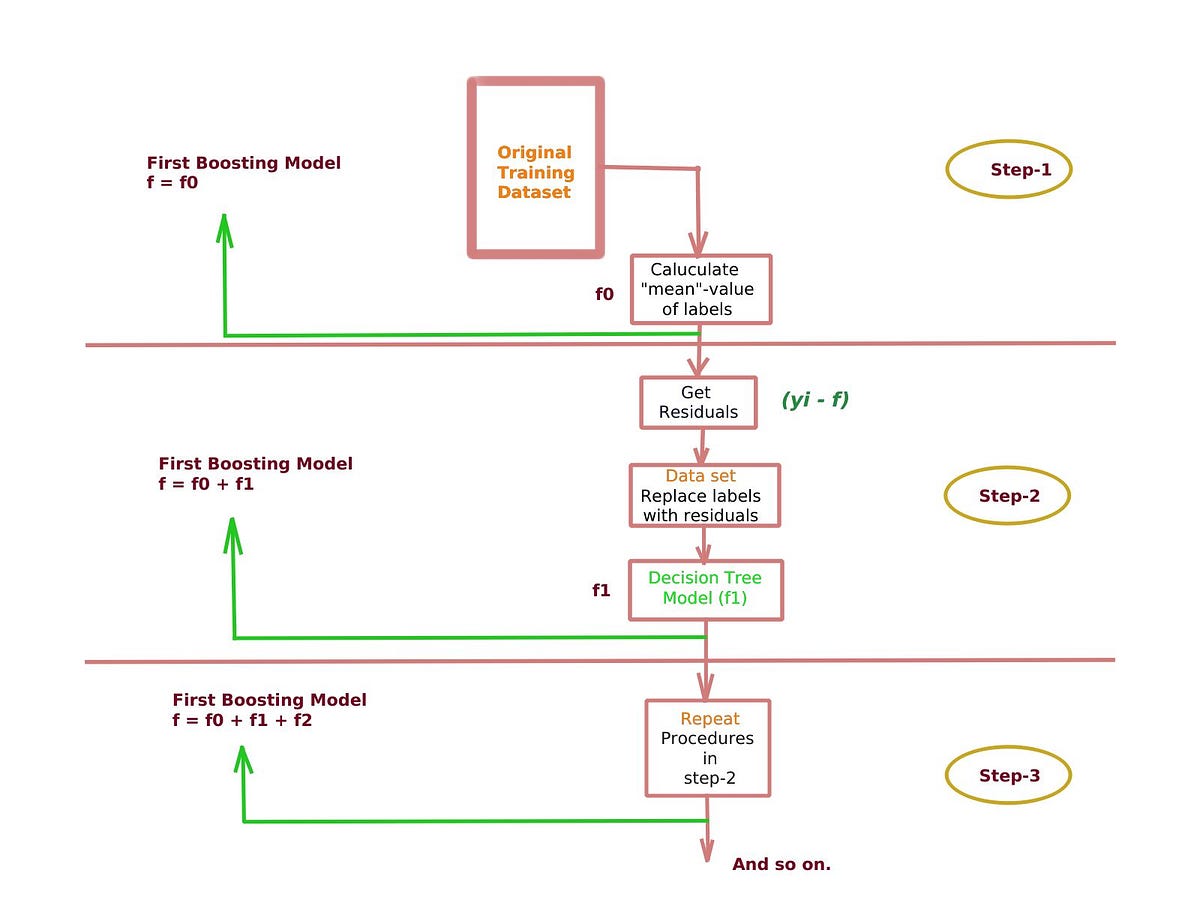
1. Building our ensemble regressor simply by starting with this constant model (𝑓=_𝑓 _0) where _𝑓 _0 is the average value of actual (observed) outputs

2. Then replace labels of each example (instance) i = 1, . . . , N in the training data set with the result of the following formula:

Where _𝑦_̂ 𝑖 , called the residual, is the new label for example 𝑥𝑖, 𝑦𝑖 is actual output and 𝑓(𝑥𝑖) is the first predicted output of boosting model (calculated mean value which is fixed through all values of X in this case).

3. Now we use the modified training set, with residuals instead of original labels, to build a new decision tree model, _𝑓_1

4. Get output of _𝑓_1 decision-tree then the boosting model is now defined as:

where 𝛼 is the learning rate (a hyper-parameter with value 0→1).

5. Repeat point-2 to get new residuals and again replace the labels in our training data set with these new residuals.

6. Build a new decision tree model, _𝑓_2 based on new data set and get results.

7. The new boosting model is now redefined as:

8. The process continues until the maximum of _𝑀 _(another hyper-parameter) trees are combined.

9. For this reason gradient boosting is called sequential model

Fig.2 Gradient Boosting Regression

So, what’s happening here? Boosting algorithm has applied the policy of reducing the residuals (errors) that results from each base-learner gradually.

#ensemble #gradient-boosting #random-forest #algorithms