In my previous post, we completed a pretty in-depth walk through of the exploratory data analysis process for a customer churn analysis dataset. Our data, sourced from Kaggle, is centered around customer churn, the rate at which a commercial customer will leave the commercial platform that they are currently a (paying) customer, of a telecommunications company, Telco. Now that the EDA process has been complete, and we have a pretty good sense of what our data tells us before processing, we can move on to building a Logistic Regression classification model which will allow for us to predict whether a customer is at risk to churn from Telco’s platform.

The complete GitHub repository with notebooks and data walkthrough can be found here.

Photo by Austin Distel on Unsplash

The Logistic Regression

When working with our data that accumulates to a binary separation, we want to classify our observations as the customer “will churn” or “won’t churn” from the platform. A logistic regression model will try to guess the probability of belonging to one group or another. The logistic regression is essentially an extension of a linear regression, only the predicted outcome value is between [0, 1]. The model will identify relationships between our target feature, Churn, and our remaining features to apply probabilistic calculations for determining which class the customer should belong to. We will be using the ‘ScikitLearn’ package in Python.

Recapping the Data

As a reminder, in our dataset we have 7043 rows (each representing a unique customer) with 21 columns: 19 features, 1 target feature (Churn). The data is composed of both numerical and categorical features, so we will need to address each of the datatypes respectively.

Target:

• Churn — Whether the customer churned or not (Yes, No)

Numeric Features:

• Tenure — Number of months the customer has been with the company
• MonthlyCharges — The monthly amount charged to the customer
• TotalCharges — The total amount charged to the customer

Categorical Features:

• CustomerID
• Gender — M/F
• SeniorCitizen — Whether the customer is a senior citizen or not (1, 0)
• Partner — Whether customer has a partner or not (Yes, No)
• Dependents — Whether customer has dependents or not (Yes, No)
• PhoneService — Whether the customer has a phone service or not (Yes, No)
• MulitpleLines — Whether the customer has multiple lines or not (Yes, No, No Phone Service)
• InternetService — Customer’s internet service type (DSL, Fiber Optic, None)
• OnlineSecurity — Whether the customer has Online Security add-on (Yes, No, No Internet Service)
• OnlineBackup — Whether the customer has Online Backup add-on (Yes, No, No Internet Service)
• DeviceProtection — Whether the customer has Device Protection add-on (Yes, No, No Internet Service)
• TechSupport — Whether the customer has Tech Support add-on (Yes, No, No Internet Service)
• StreamingTV — Whether the customer has streaming TV or not (Yes, No, No Internet Service)
• StreamingMovies — Whether the customer has streaming movies or not (Yes, No, No Internet Service)
• Contract — Term of the customer’s contract (Monthly, 1-Year, 2-Year)
• PaperlessBilling — Whether the customer has paperless billing or not (Yes, No)
• PaymentMethod — The customer’s payment method (E-Check, Mailed Check, Bank Transfer (Auto), Credit Card (Auto))

Preprocessing Our Data For Modeling

We moved our data around a bit during the EDA process, but that pre-processing was mainly for ease of use and digestion, rather than functionality for a model. For the purposes of our Logistic Regression, we must pre-process our data in a different way, particularly to accommodate the categorical features which we have in our data. Let’s take a look at our data info one more time to get a sense of what we are working with.

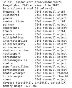
We do not have any missing data and our data-types are in order. Note that the majority of our data are of ‘object’ type, our categorical data. This will be our primary area of focus in the preprocessing step. At the top of the data, we see two columns that are unnecessary, ‘Unnamed: 0’ and ‘customerid’. These two columns will be irrelevant to our data, as the former does not have any significant values and the latter is a unique identifier of the customer which is something we do not want. We quickly remove these features from our DataFrame via a quick pandas slice:

df2 = df.iloc[:,2:]

The next step is addressing our target variable, Churn. Currently, the values of this feature are “Yes” and “No”. This is a binary outcome, which is what we want, but our model will not be able to meaningfully interpret this in its current string-form. Instead, we want to replace these variables with numeric binary values:

df2.churn.replace({"Yes":1, "No":0}, inplace = True)

Up next, we must deal with our remaining categorical variables. A Dummy Variable is a way of incorporating nominal variables into a regression as a binary value. These variables allow for the computer to interpret the values of a categorical variable as high(1) or low(0) scores. Because the variables are now numeric, the model can assess directionality and significance in our variables instead of trying to figure out what “Yes” or “No” means. When adding dummy variables is performed, it will add new binary features with [0,1] values that our computer can now interpret. Pandas has a simple function to perform this step.

dummy_df = pd.get_dummies(df2)

**Note: **It is very important to pay attention to the “drop_first” parameter when categorical variables have more than binary values. We cannot use all values of categorical variables as features because this would raise the issue of multicollinearity (computer will place false significance on redundant information) and break the model. We must leave one of the categories out as a reference category.

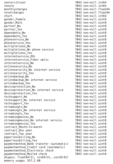
Our new DataFrame features are above and now include dummy variables.

Splitting our Data

We must now separate our data into a target feature and predicting features.

# Establish target feature, churn
y = dummy_df.churn.values

# Drop the target feature from remaining features
X = dummy_df.drop('churn', axis = 1)
# Save dataframe column titles to list, we will need them in next step
cols = X.columns

Feature Scaling

Our data is almost fully pre-processed but there is one more glaring issue to address, scaling. Our data is full of numeric data now, but they are all in different units. Comparing a binary value of 1 for ‘streamingtv_Yes’ with a continuous price value of ‘monthlycharges’ will not give any relevant information because they have different units. The variables simply will not give an equal contribution to the model. To fix this problem, we will standardize our data values via rescaling an original variable to have equal range & variance as the remaining variables. For our purposes, we will use Min-Max Scaling [0,1] because the standardize value will lie within the binary range.

#machine-learning #customer-churn #data-science #logistic-regression #data-analysis