This is the thirteenth article of my column Mathematical Statistics and Machine Learning for Life Sciences where I try to explain some mysterious analytical techniques used in Bioinformatics, Biomedicine, Genetics etc. in a simple way. In the previous post How Exactly UMAP works I started with an intuitive explanation of the math behind UMAP. The best way to learn it is to program UMAP from scratch, this is what we are going to do today. The idea of this post is to show that it is relatively easy for everyone to create their own neighbor graph dimension reduction technique that can provide even better visualization than UMAP. It is going to be lots of coding, buckle up!
Building High-Dimensional Probabilities
As a test data set, we will be using the Cancer Associated Fibroblasts (CAFs) scRNAseq data. We start with importing Python libraries (mainly numpy and scikit-learn will be used), having a look at the data matrix and checking the dimensions of the data set. Please note, that the rows are cells and columns are genes here, the last column contains the coding of the clustering results, i.e. each cell belongs to one of 4 clusters with IDs #1, 2, 3 and 4:
import numpy as np
import pandas as pd
import matplotlib.pyplot as plt
from sklearn.metrics.pairwise import euclidean_distances

expr = pd.read_csv('CAFs.txt', sep='\t')
X_train = expr.values[:,0:(expr.shape[1]-1)]
X_train = np.log(X_train + 1)
n = X_train.shape[0]
print("\nThis data set contains " + str(n) + " samples")
y_train = expr.values[:,expr.shape[1]-1]
print("\nDimensions of the  data set: ")
print(X_train.shape, y_train.shape)
One important global variable to define from the very beginning is the matrix of squared pairwise Euclidean distances for the initial high-dimensional scRNAseq data set, this matrix will be used a lot in the future code. Here, we also define the local connectivity parameter rho, as a distance to the first nearest neighbor, see the previous post for more detailed explanations of the meaning of the parameter.
dist = np.square(euclidean_distances(X_train, X_train))
rho = [sorted(dist[i])[1] for i in range(dist.shape[0])]
print(dist[0:4, 0:4])
print('\n')
print(rho[0:4])
Using the matrix of squared pairwise Euclidean distances we will compute the matrix of probabilities in the high-dimensional space. Knowing the matrix, we can easily calculate the Entropy as a sum of probabilities for each cell, and the number of nearest neighbors, k, as k = 2^Entropy. Please note the argument σ of the function. This implies that the matrix of probabilities as a function of σ will be used later for the binary search procedure that computes the optimal σ for the fixed number of nearest neighbors.
prob_high_dim.py
def prob_high_dim(sigma, dist_row):
    """
    For each row of Euclidean distance matrix (dist_row) compute
    probability in high dimensions (1D array)
    """
    d = dist[dist_row] - rho[dist_row]; d[d < 0] = 0
    return np.exp(- d / sigma)

def k(prob):
    """
    Compute n_neighbor = k (scalar) for each 1D array of high-dimensional probability
    """
    return np.power(2, np.sum(prob))
A trick here is that for convenience we compute a 1D array of probabilities for each i-th cell, this means for each i-th row (or column) of the squared pairwise Euclidean distance matrix (distance from i-th cell to all other cells in the data set). This is done because of the unknown σ_i in the equation:

We have to use binary search in order to find σ_i for each i-th cell in the data set. For each i-th cell, given the 1D array of the high-dimensional probabilities, we can sum up the elements of the array and compute the number of nearest neighbors, k, according to the definition:

So now we have a function that produces the number of nearest neighbors, k, (scalar) value for each σ i_ for each i-th cell. We can fix the number of nearest neighbors value (desired k hyper-parameter) and input this function into the binary search procedure in order to compute the σ_i for each i-th cell.
binary_search.py
def sigma_binary_search(k_of_sigma, fixed_k):
    """
    Solve equation k_of_sigma(sigma) = fixed_k
    with respect to sigma by the binary search algorithm
    """
    sigma_lower_limit = 0; sigma_upper_limit = 1000
    for i in range(20):
        approx_sigma = (sigma_lower_limit + sigma_upper_limit) / 2
        if k_of_sigma(approx_sigma) < fixed_k:
            sigma_lower_limit = approx_sigma
        else:
            sigma_upper_limit = approx_sigma
        if np.abs(fixed_k - k_of_sigma(approx_sigma)) <= 1e-5:
            break
    return approx_sigma

N_NEIGHBOR = 15
prob = np.zeros((n,n)); sigma_array = []
for dist_row in range(n):
    func = lambda sigma: k(prob_high_dim(sigma, dist_row))
    binary_search_result = sigma_binary_search(func, N_NEIGHBOR)
    prob[dist_row] = prob_high_dim(binary_search_result, dist_row)
    sigma_array.append(binary_search_result)
    if (dist_row + 1) % 100 == 0:
        print("Sigma binary search finished {0} of {1} cells".format(dist_row + 1, n))
print("\nMean sigma = " + str(np.mean(sigma_array)))
Computing σ_i for each cell we get n-cells 1D arrays of probabilities, they all together build a matrix of high-dimensional probabilities. This matrix has to satisfy the symmetry condition according to the UMAP algorithm:

However, to my experience the following simpler symmetry condition provides a better visualization as we will see later.
P_symmetr.py
#P = prob + np.transpose(prob) - np.multiply(prob, np.transpose(prob))
P = (prob + np.transpose(prob)) / 2
I encourage the readers to play with different ways of obtaining the symmetric matrix of high-dimensional probabilities and check how the final visualization changes.
Building Low-Dimensional Probabilities
Next, we are going to compute the layout for the high-dimensional neighbor graph, i.e. the matrix of low-dimensional probabilities according to the UMAP definition:

Since the goal of the UMAP algorithm is to find the optimal coordinates of the low-dimensional embeddings, y_i, which are updated through the Gradient Descent procedure, I would expect that the a and b parameters should also be updated at each Gradient Descent iteration. However, in the original UMAP algorithm, they seem to be fixed at the very beginning for a desired value of min_dist hyper-parameter:
min_dist.py
MIN_DIST = 0.25

x = np.linspace(0, 3, 300)

def f(x, min_dist):
    y = []
    for i in range(len(x)):
        if(x[i] <= min_dist):
            y.append(1)
        else:
            y.append(np.exp(- x[i] + min_dist))
    return y

dist_low_dim = lambda x, a, b: 1 / (1 + a*x**(2*b))

p , _ = optimize.curve_fit(dist_low_dim, x, f(x, MIN_DIST))

a = p[0]
b = p[1]
print("Hyperparameters a = " + str(a) + " and b = " + str(b))
Again, here I see a room for improvements and experiments. For simplicity, below I will set a=1 and b=1 in order to get a sort of hybrid of UMAP and tSNE. Then the matrix of low-dimensional probabilities is given by:
prob_low_dim.py
def prob_low_dim(Y):
    """
    Compute matrix of probabilities q_ij in low-dimensional space
    """
    inv_distances = np.power(1 + a * np.square(euclidean_distances(Y, Y))**b, -1)
    return inv_distances
Learning Low-Dimensional Embeddings
Finally, we are going to code the cost function of UMAP which is the Cross-Entropy, please see the previous post for details of how this cost function is capable of preserving global distances. We are actually interested not in the Cross-Entropy itself but in its gradient to be used in the Gradient Descent procedure later.
cross_entropy.py
def CE(P, Y):
    """
    Compute Cross-Entropy (CE) from matrix of high-dimensional probabilities
    and coordinates of low-dimensional embeddings
    """
    Q = prob_low_dim(Y)
    return - P * np.log(Q + 0.01) - (1 - P) * np.log(1 - Q + 0.01)

def CE_gradient(P, Y):
    """
    Compute the gradient of Cross-Entropy (CE)
    """
    y_diff = np.expand_dims(Y, 1) - np.expand_dims(Y, 0)
    inv_dist = np.power(1 + a * np.square(euclidean_distances(Y, Y))**b, -1)
    Q = np.dot(1 - P, np.power(0.001 + np.square(euclidean_distances(Y, Y)), -1))
    np.fill_diagonal(Q, 0)
    Q = Q / np.sum(Q, axis = 1, keepdims = True)
    fact=np.expand_dims(a*P*(1e-8 + np.square(euclidean_distances(Y, Y)))**(b-1) - Q, 2)
    return 2 * b * np.sum(fact * y_diff * np.expand_dims(inv_dist, 2), axis = 1)
Please note the Q matrix in the CE_gradient function. It is not supposed to be normalized according to the UMAP algorithm. However, to my experience this normalization improves the low-dimensional visualization. I encourage again everyone to experiment here. Finally, we initialize the coordinates of low-dimensional embeddings y_i with Graph Laplacian and launch the Gradient Descent procedure:
grad_descent.py
N_LOW_DIMS = 2
LEARNING_RATE = 1
MAX_ITER = 200

np.random.seed(12345)
model = SpectralEmbedding(n_components = N_LOW_DIMS, n_neighbors = 50)
y = model.fit_transform(np.log(X_train + 1))
#y = np.random.normal(loc = 0, scale = 1, size = (n, N_LOW_DIMS))

CE_array = []
print("Running Gradient Descent: \n")
for i in range(MAX_ITER):
    y = y - LEARNING_RATE * CE_gradient(P, y)

    plt.figure(figsize=(20,15))
    plt.scatter(y[:,0], y[:,1], c = y_train.astype(int), cmap = 'tab10', s = 50)
    plt.title("UMAP on Cancer Associated Fibroblasts (CAFs): Programmed from Scratch",
              fontsize = 20)
    plt.xlabel("UMAP1", fontsize = 20); plt.ylabel("UMAP2", fontsize = 20)
    plt.savefig('UMAP_Plots/UMAP_iter_' + str(i) + '.png')
    plt.close()

    CE_current = np.sum(CE(P, y)) / 1e+5
    CE_array.append(CE_current)
    if i % 10 == 0:
        print("Cross-Entropy = " + str(CE_current) + " after " + str(i) + " iterations")

plt.figure(figsize=(20,15))
plt.plot(CE_array)
plt.title("Cross-Entropy", fontsize = 20)
plt.xlabel("ITERATION", fontsize = 20); plt.ylabel("CROSS-ENTROPY", fontsize = 20)
plt.show()

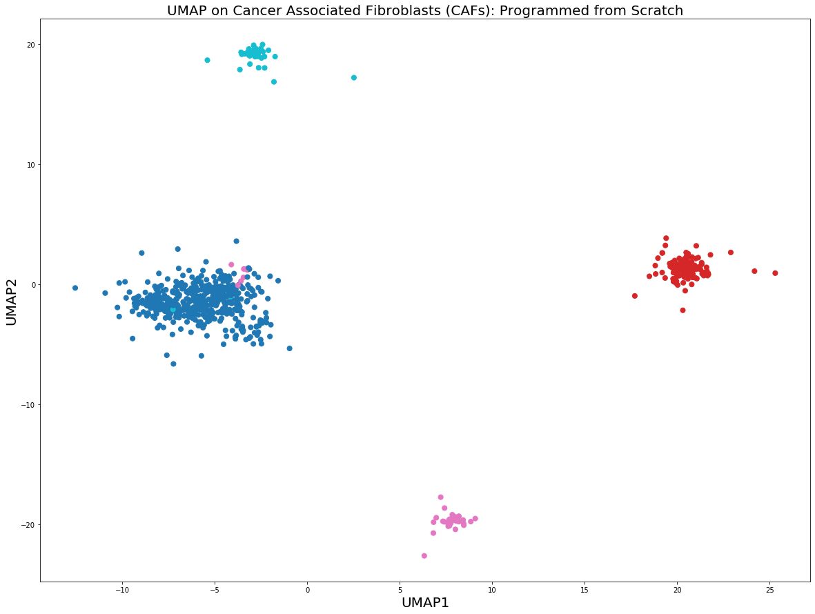
The Cross Entropy seems to be decreasing and reaching a plateau. Please note that here for simplicity I implement the regular Gradient Descent rather than Stochastic Gradient Descent that is used by the original implementation of UMAP. This is because the goal of the post is to demonstrate the idea of UMAP and not to provide an optimized and pretty code. Now, we can visualize the low-dimensional embeddings:
plot_UMAP.py
plt.figure(figsize=(20,15))
plt.scatter(y[:,0], y[:,1], c = y_train.astype(int), cmap = 'tab10', s = 50)
plt.title("UMAP on Cancer Associated Fibroblasts (CAFs): Programmed from Scratch",
          fontsize = 20)
plt.xlabel("UMAP1", fontsize = 20); plt.ylabel("UMAP2", fontsize = 20)
plt.show()

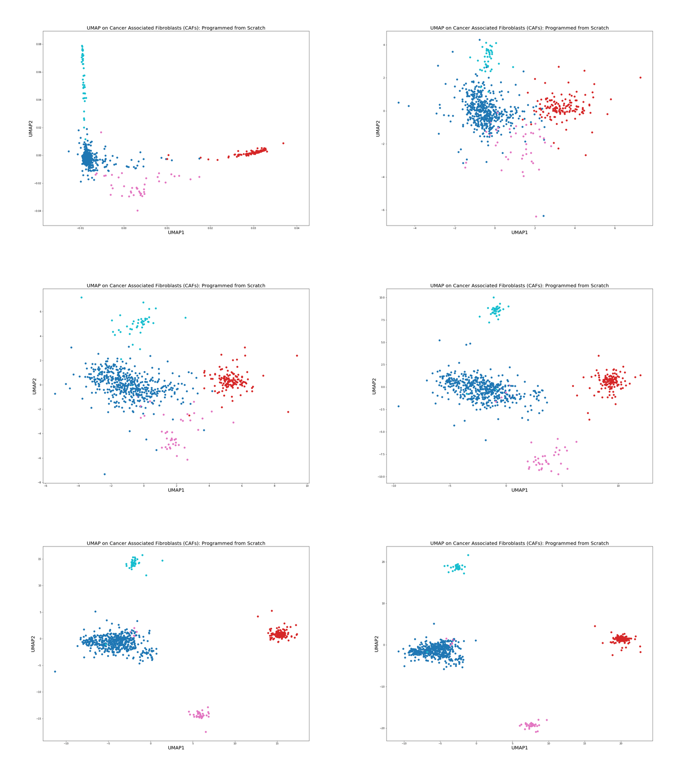
We can also easily animate how the distinct clusters are formed starting from the Laplacian embeddings, this is done by merging plots from each iteration into a gif-file.
convert -delay 0 $(for i in $(seq 0 1 20; seq 21 10 199); do echo UMAP_iter_${i}.png; done) \
-loop 0 UMAP_animated.gif

The from scratch implementation of UMAP seems to be working fine, the clusters of the 4 cell populations are clearly distinguishable. Clustering algorithms would not have problems identifying the cell populations if we were to run them on the low-dimensional embeddings above.
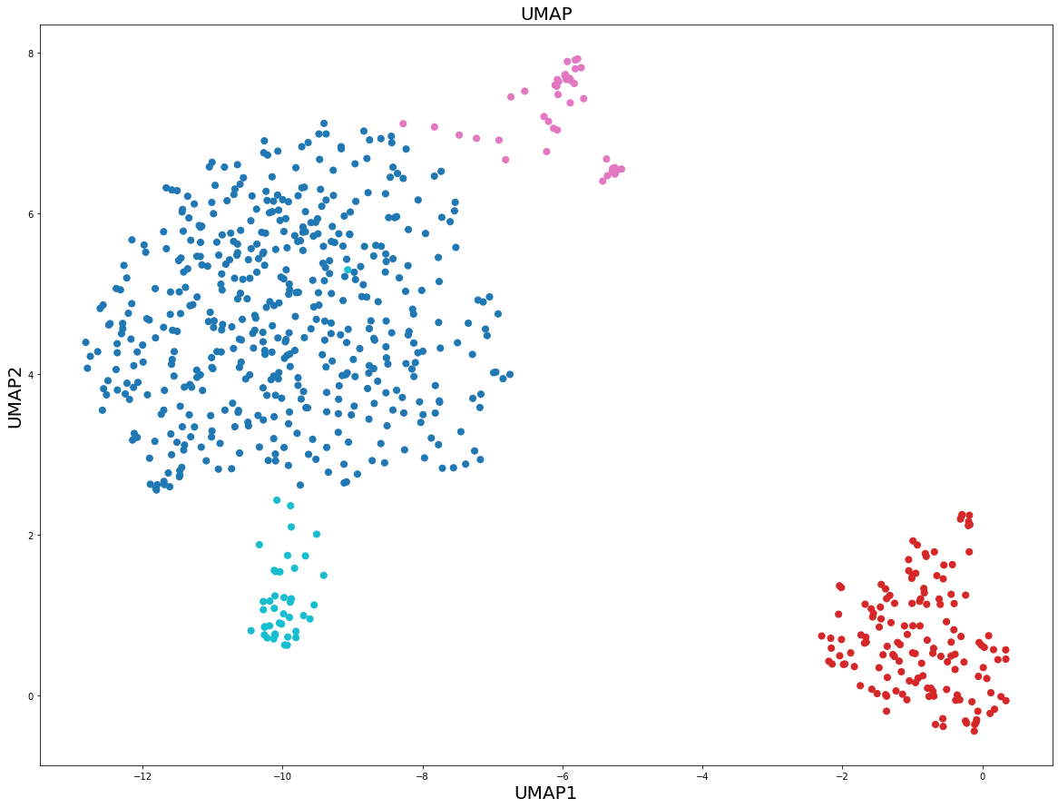
Let us compare the figure above with the original UMAP Python + numba implementation. We are going to use n_neighbors = 15 and min_dist = 0.25, i.e. identical values of UMAP hyperparameters as in the previous from scratch UMAP implementation.
original_UMAP.py
from umap import UMAP
plt.figure(figsize=(20,15))
model = UMAP(n_neighbors = 15, min_dist = 0.25, n_components = 2, verbose = True)
umap = model.fit_transform(X_train)
plt.scatter(umap[:, 0], umap[:, 1], c = y_train.astype(int), cmap = 'tab10', s = 50)
plt.title('UMAP', fontsize = 20)
plt.xlabel("UMAP1", fontsize = 20)
plt.ylabel("UMAP2", fontsize = 20)
plt.show()

What we can see here is that in a sense the from scratch implementation gives more distinct clusters compared to the original UMAP implementation. This is due to small changes applied on the way, such as slightly different symmetry condition and normalization of the Q matrix in the gradient of Cross Entropy.
Summary
In this post, we have learnt that it is relatively easy to implement UMAP from scratch in Python. Therefore, my prediction is that UMAP is just the beginning, and there going to be many more, and possibly better, dimension reduction techniques appearing in the Single Cell Genomics research area in the nearest future. It is quite straightforward to tune the low- and high-dimensional distributions, make better normalization and symmetry conditions, better cost functions, and play with attractive / repulsive forces for the N-body problem in order to get even better low-dimensional representations.
In the comments below let me know which analytical techniques in Life Sciences seem especially mysterious to you and I will try to cover them in the future posts. Check the codes from the post on my github. Follow me at Medium Nikolay Oskolkov, in Twitter @NikolayOskolkov and connect in Linkedin. Next time I will turn to Evolutionary Biology and show how to estimate population size back in time using Ancient DNA, stay tuned.
#DeepLearning # machine learning #TensorFlow
