This chapter continues the series on Bayesian deep learning. In the chapter we’ll explore alternative solutions to conventional dense neural networks. These alternatives will invoke probability distributions over each weight in the neural network resulting in a single model that effectively contains an infinite ensemble of neural networks trained on the same data. We’ll use this knowledge to solve an important problem of our age: how long to boil an egg.

Chapter Objectives:

• Become familiar with variational inference with dense Bayesian models
• Learn how to convert a normal fully connected (dense) neural network to a Bayesian neural network
• Appreciate the advantages and shortcomings of the current implementation

The data is from an experiment in egg boiling. The boil durations are provided along with the egg’s weight in grams and the finding on cutting it open. Findings are categorised into one of three classes: under cooked, soft-boiled and hard-boiled. We want the egg’s outcome from its weight and boiling time. The problem is insanely simple, so much so that the data is near being linearly separable¹⁠. But not quite, as the egg’s pre-boil life (fridge temperature or cupboard storage at room temperature) aren’t provided and as you’ll see this swings cooking times. Without the missing data we can’t be certain what we’ll find when opening an egg up. Knowing how certain we are we can influence the outcome here as we can with most problems. In this case if relatively confident an egg’s undercooked we’ll cook it more before cracking it open.

Let’s have a look at the data first to see what we’re dealing with. If you want to feel the difference for yourself you can get the data at github.com/DoctorLoop/BayesianDeepLearning/blob/master/egg_times.csv. You’ll need Pandas and Matplotlib for exploring the data. (pip install — upgrade pandas matplotlib) Download the dataset to the same directory you’re working from. From a Jupyter notebook type pwd on its own in a cell to find out where that directory is if unsure.

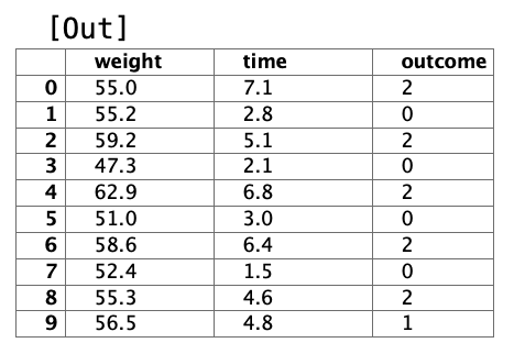
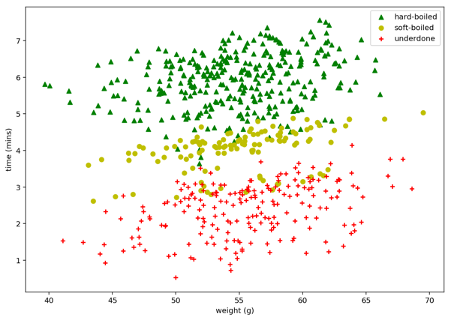
Figure 2.01 Scatter plot of egg outcomes

And let’s see it now as a histogram.

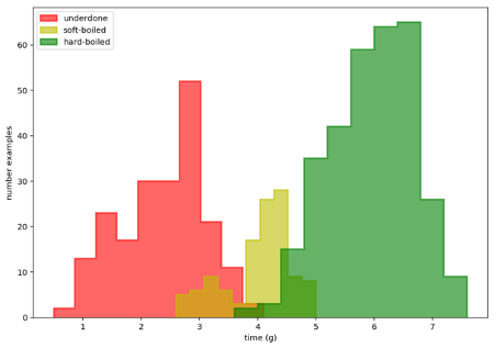
Figure 2.02 Histogram of egg times by outcome

It seems I wasn’t so good at getting my eggs soft-boiled as I like them so we see a fairly large class imbalance with twice as many underdone instances and three times as many hardboiled instances relative to the soft-boiled lovelies. This class imbalance can spell trouble for conventional neural networks causing them to underperform and an imbalanced class size is a common finding.

Note that we’re not setting density to True (False is the default so doesn’t need to be specified) as we’re interested in comparing actual numbers. While if we were comparing probabilities sampled from one of the three random variables, we’d want to set density=True to normalise the histogram summing the data to 1.0.

#editors-pick #bayesian-machine-learning #deep-learning #bayesian-neural-network #neural-networks #deep learning