Sub-plotting is a very powerful feature in MATLAB. They allow users to very quickly create customized data visualizations and displays. They can also be used to quickly create interactive Graphical User Interfaces (GUIs). In this tutorial, I describe three different ways to use the subplot() command and provide examples of each. The provided examples work in both MATLAB and Octave.

The source code for the included examples can be found in the GitHub repository.

Using Basic Subplots

The subplot() function in MATLAB/Octave allows you to insert multiple plots on a grid within a single figure. The basic form of the subplot() command takes in three inputs: nRows, nCols, linearIndex. The first two arguments define the number of rows and columns that will be included in the grid. The third argument is a linear index that selects the current active plot axes. The index starts at 1 and increases from left to right and top to bottom. It’s OK if this doesn’t make sense yet, the ordering is visualized in all of the examples within this section, and is especially obvious in the grid example.

Let’s start with a simple example that includes three sub-plots along a single row. For convenience, I have also used the text() function to display the linear index in each subplot.

a1 = subplot( 1, 3, 1 );
text( 0.5, 0.5, '1', 'fontsize', 48 );
a2 = subplot( 1, 3, 2 );
text( 0.5, 0.5, '2', 'fontsize', 48 );
a3 = subplot( 1, 3, 3 );
text( 0.5, 0.5, '3', 'fontsize', 48 );

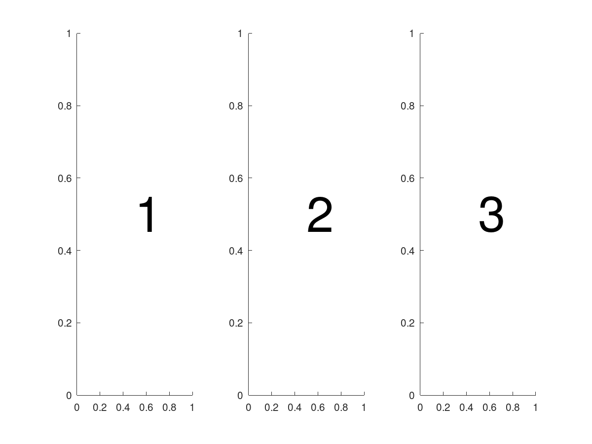
Image by author

Notice in the code for this example that I have saved the axes handle (a1, a2, a3) for each of the subplots. This is important because now that there are multiple plot axes on the figure, we will need to specify which axes we are referencing whenever we change properties. For example, if we wanted to change the font size, we would have to specify the font size on each axes. The code snippet below is an example where the font is being set to a different size on each axes. This concept extends to all other plot axes properties and shows how each sub-plot can be fully customized.

set( a1, 'fontsize', 12 )
set( a2, 'fontsize', 14 )
set( a3, 'fontsize', 16 )

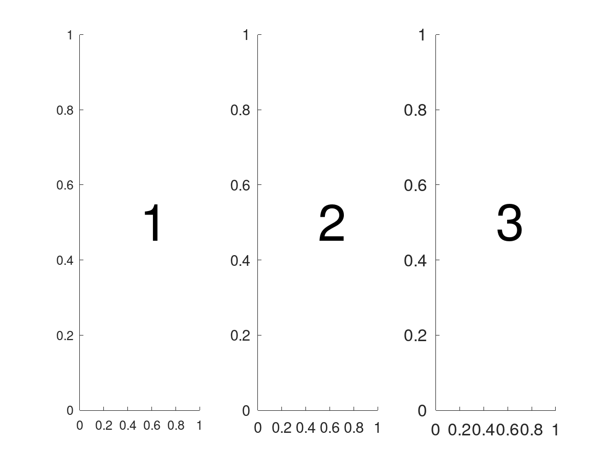
Image by author

Here is another example where I have swapped the first two arguments in the subplot function and now we will create a figure with three rows.

a1 = subplot( 3, 1, 1 );
text( 0.5, 0.5, '1', 'fontsize', 48 );
a2 = subplot( 3, 1, 2 );
text( 0.5, 0.5, '2', 'fontsize', 48 );
a3 = subplot( 3, 1, 3 );
text( 0.5, 0.5, '3', 'fontsize', 48 );

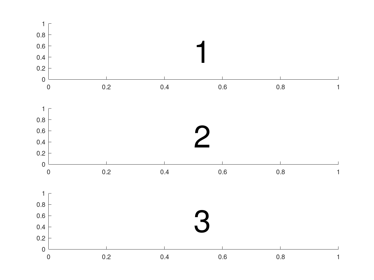
Image by author

Finally, we can create a full grid of sub-plots. In this example, I have included 3 rows and 3 columns; however, any combination can be used. This example nicely illustrates how the linear index increases.

for iPlot=1 : 9
  subplot( 3, 3, iPlot );
  text( 0.5, 0.5, num2str( iPlot ), 'fontsize', 48 );
end

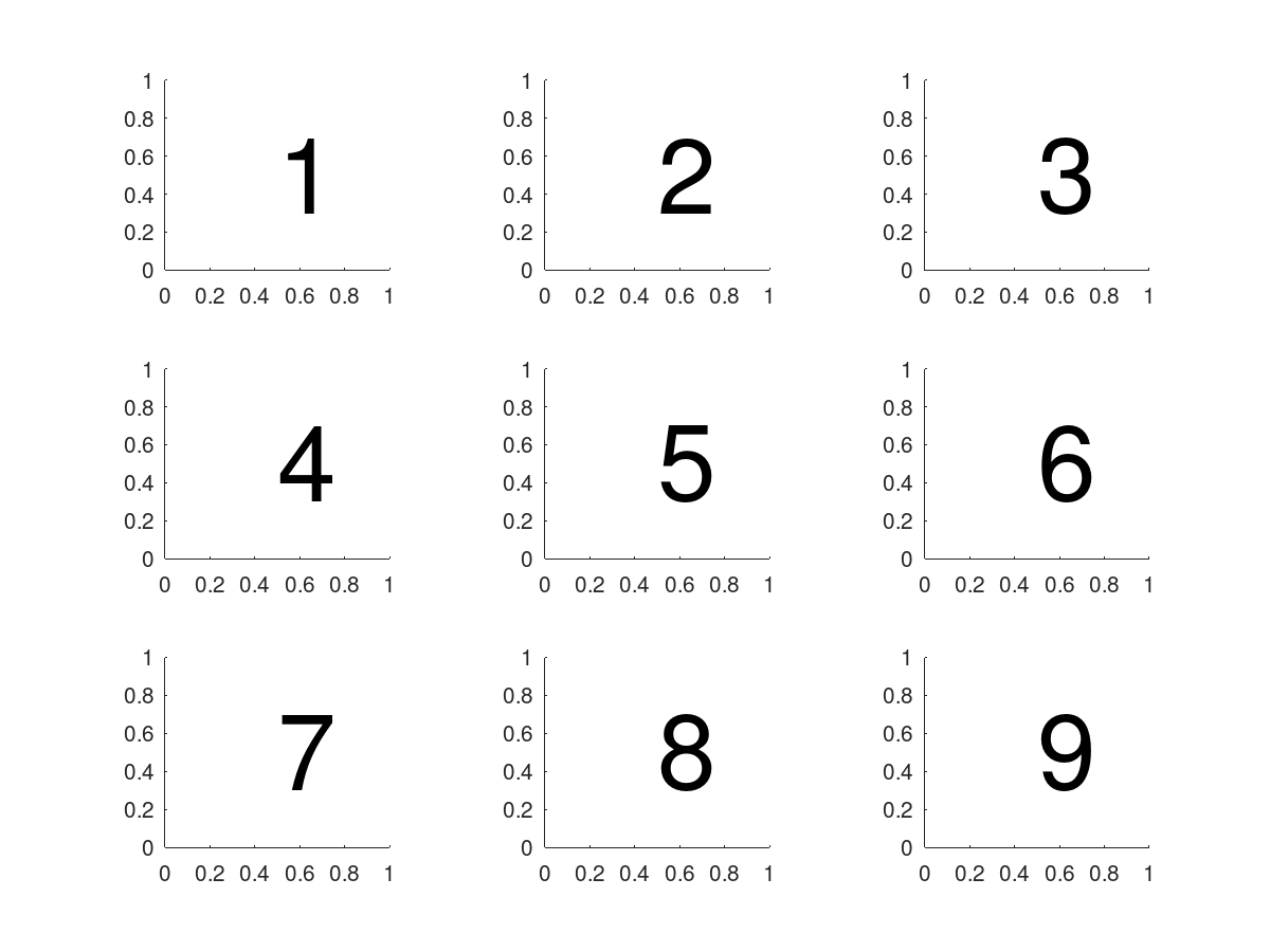
Image by author

Using Different Sized Plots

A slightly more flexible way of using subplot() is to place sub-plots over multiple points in the grid. This is accomplished by passing in an array of linear indices as third argument, rather than just a single value. So for example, subplot( 1, 3, [1, 2] ) would create a subplot grid that has three columns and a single plot that occupies the first two columns. This method lets you make some really nice looking plots that can easily accommodate various types of data.

Let’s look at another example. The underlying grid is of shape 3 x 3. The first sub-plot is placed at the top of the grid and spans all three columns. The second sub-plot is placed in the bottom left corner and covers a 2 x 2 sub-grid. Finally, the last sub-plot is in the bottom right corner and spans the last two rows. In all cases, the linear indices have been included over the plots to illustrate which parts of the grid they are covering.

% - Create a single plot on the top row
subplot( 3, 3, 1:3 );
text( 0.35, 0.5, '1, 2, 3', 'fontsize', 48 );
% - Create a single plot in the last column
subplot( 3, 3, [6, 9] );
text( 0.30, 0.5, '6, 9', 'fontsize', 48 );
% - Create a matrix in the bottom left corner
subplot( 3, 3, [ 4:5, 7:8 ] );
text( 0.25, 0.5, '4, 5, 7, 8', 'fontsize', 48 );

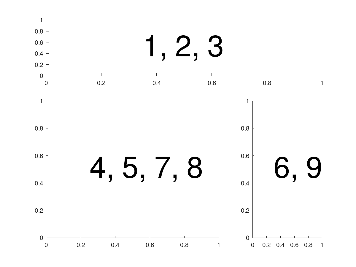
Image by author

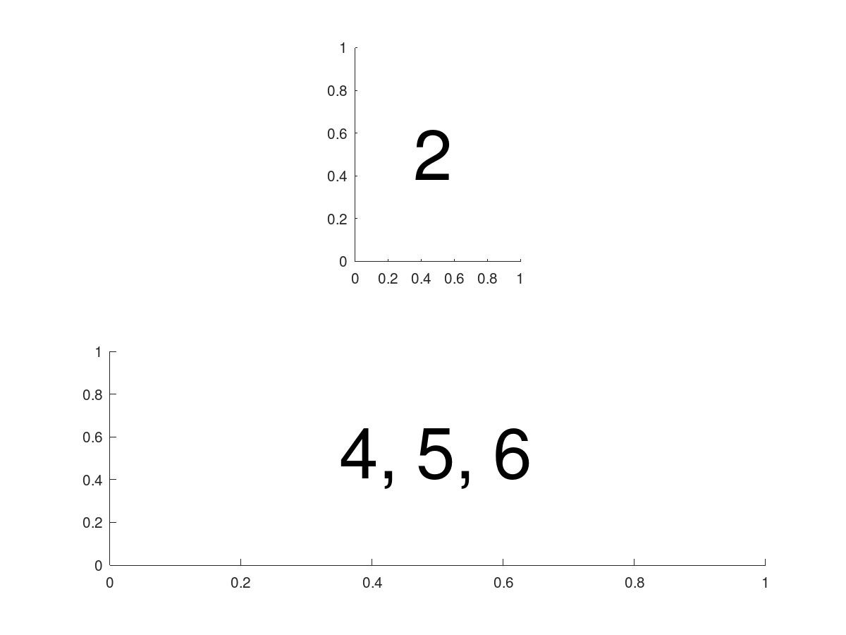
Another convenient use of populating large grids is to simply leave some empty. This is nice because it creates white space and allows you to align sub-plots at different places within the figure. Here is an example that centers a sub-plot in the top row and spans the sub-plot in the bottom row across all of the columns.

subplot( 2, 3, 2 );
text( 0.35, 0.5, '2', 'fontsize', 48 );
subplot( 2, 3, 4:6 );
text( 0.35, 0.5, '4, 5, 6', 'fontsize', 48 );

#octave #coding #matlab #visual studio code