In the second part of this series, we will discuss how the neural network learns through forward and backward propagation to update the weights and biases to fit to the training data. These can then be used to predict future data that it has not seen before.

In Part 1 — Using the right dimensions for your Neural Network, we discussed how to choose a consistent convention for the vector and matrix shapes in your neural network architecture. While different software implementation may use a different convention, having a solid understanding makes it easy to know what preprocessing may be needed to fit the module design.

Using the right dimensions for your Neural Network

[When building your Artificial Neural Networks, one of the frustrating bugs is getting the shape of the vectors and…]

In this part, we are going to extend our knowledge to understand how a neural network learns through the training sets provided. We will use a single-hidden layer neural network in this article to illustrate the key concepts below:

• Linear functions, and non-linear activation functions
• Start the ball rolling using random initialisation of the weights and biases
• Use forward propagation to compute the prediction
• Use a Loss Function to compute how far off we were from the ground truth
• Use back propagation to nudge each of the weights and biases closer to the truth
• Rinse and repeat — it’s as simple as that!

In this article, we will build a simple binary classifier architecture to predict whether images show that of a cat, or non-cat (for some reasons, someone starting out ML years ago must love cats — many examples you see involve these cute animals!)

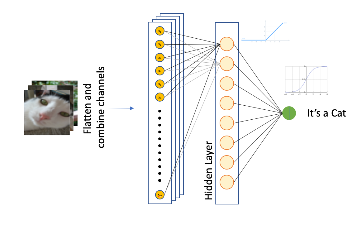
Overall single-layer architecture

Quick overview of architecture

The original shape of the training set is (209, 64, 64, 3), representing 3-channel 64-by-64 images of cats and non-cats. The Google Colab script to explore the data can be found below, though this article will not go into the full code to build the feed forward neural network. We will cover the code implementation in the next article.

Read and explore the training data set

In the last two code blocks, we reduced the dimensionality to a single black-and-white channel instead to keep it simple. In a future article, we will explore how Convolutional Neural Networks (CNNs) are better at image recognition tasks as it retains the pixel relationship across the 2-dimensions of the image. For now, we will flatten the images across the training set, resulting in an input matrix with shape (64*64, 209).

Number of trainable parameters

For each training example, the input comprises 4096 features each representing a pixel in the original picture.

The hidden layer is made up of 8 neurons. Recalling our convention in Part 1, the weights matrix has a shape of (8, 4096) and the bias vector has a shape of (8, 1). In total, the hidden layer of this simple neural network has a total of (8 * 4096) + 8 = 32,776 trainable parameters.

The output layer comprises a single node, and thus the weights matrix for the output node is with a shape of (1, 8), resulting in 9 trainable parameters (8 weights and 1 bias).

This model thus has a total of 32776 + 9 = 32,785 parameters that can be trained.

---

Each neuron will have both a linear function of the form z = wᵢxᵢ + b, with i representing values from 1 to 4096 in our example above. Each of this result is then passed to a non-linear activation function g(z).

This results in a vector with shape (8, 209) in our example, which will be fed into the output layer. The output layer in our example is a single node that performs a binary classification.

Let’s now walk through the key concepts to understand how the neural network learns through this architecture.

#artificial-intelligence #machine-learning #deep-learning #data-science #deep learning