This article will introduce key concepts about Regularized Loss Minimization (RLM) and Empirical Risk Minimization (ERM), and it’ll walk you through the implementation of the least-squares algorithm using MATLAB. The models obtained using RLM and ERM will then be compared and discussed against each other.

We’ll use a polynomial curve-fitting problem to predict the best polynomial for this data. The least-squares algorithm will be implemented step-by-step using MATLAB.

By the end of this post, you’ll understand the least-squares algorithm and be aware of the advantages and downsides of RLM and ERM. Additionally, we’ll discuss some important concepts about overfitting and underfitting.

Dataset

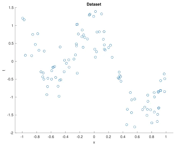
We’ll use a simple one input dataset with N = 100 data points. This dataset was originally proposed by Dr. Ruth Urner on one of her assignments for a machine learning course. In the repository below, you’ll find two TXT files: dataset1_inputs.txt and dataset1_outputs.txt.

These files contain the input and output vectors. Using MATLAB, we’ll plot these data points in a chart. On MATLAB, I imported them in Home > Import Data. Then, I created the flowing script for plotting the data points.

#data-science #programming #polynomial-regression #least-squares #machine-learning