An In-Depth Analysis Of The Space-Partitioning Data Structure

By now you’d have come across many articles on the K-Nearest Neighbor algorithm. Be it a basic image classifier, or a simple movie recommender app for home entertainment, or even, looking up the nearest gas station on your phone, you’ll find the k-NN algorithm in action. It is the simplest algorithmic tool that works well for classification, regression, and mapping applications.

Like any other algorithm, the nearest neighbor also has a brute-force method that isn’t practical for any real application. The alternative is to use efficient data structures like the k-dimensional tree or the ball-tree as a foundation for the search algorithm.

In this post, we’ll focus on learning the k-dimensional tree along with basic operations to manipulate its data.

Before we dive in, let’s do a quick recap of trees and some of its common variants.

Trees: A Quick Recap

Formally, a tree is defined as a finite set of one or more nodes such that:

• There is a designated node called the root.
• The remaining nodes are partitioned into n ≥ 0 disjoint sets T₁, ……, Tₙ where each of these sets is a tree and called sub-trees of the root. ₁

For example, say, you have a set Α = {8, 9, 4, 1, 3, 5, 10, 7, 2, 6}. If you choose the root to be 8 and the number of partitions n = 9, then, by definition, the remaining nodes in the set form independent sub-trees.

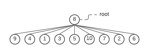
A tree with root=8 and nine sub-trees . ~Image by author

If you choose n = 3 as the number of partitions, you’ll end up with three disjoint subsets: Β = {9, 4, 1}, Γ = {3, 5, 10}, and Δ = {7, 2, 6}. Once again, each subset has a node as its root.

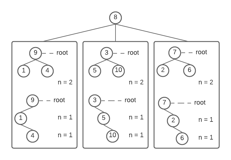
Top-half: With n = 2, each root has two children that are themselves root nodes. Bottom-half: With n = 1, each root has one child that intern has a root and a child node. ~Image by author

The root nodes 9, 3, 7 from the sub-trees form equal children of node 8. Each sub-tree can be further partitioned into 1 or 2 sub-trees. The above figure shows this in detail.

Binary Trees

A binary tree is an important tree structure you come across quite often. It is defined as a finite set of nodes that is empty or consists of a root and the left and the right sub-trees. ₁

Binary Search Trees

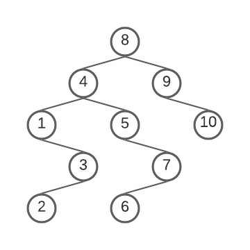
A Binary Search Tree created from the set Α. ~Image by author

An important use-case of the binary tree is the_ Binary Search Tree_ (BST).

Take a look at this tree for example. Any given node in the tree has a value that is greater than its left sub-tree but less than its right sub-tree. This unique property allows us to search, insert, or delete a node in O(log(n)) time.

At a high level, a kd-tree is a generalization of a BST that stores k-dimensional points. ₂

With the prerequisites done, let’s focus on the concept of the kd-tree.

KD-Trees: The Concept

Developed by Jon Bentley, the kd-tree is a variation of the BST. The difference is that each level of the tree branches based on a particular dimension associated with that level. ₃

In other words, for a kd-tree with n levels, each level i, ∀ _i _= {1, … , n}, has a particular dimension _d = i mod k _assigned for comparison, called the splitting dimension. As you traverse the tree, you compare nodes at the splitting dimension of the given level. If it compares less, you branch left. Otherwise, you branch right. This preserves the structure of the BST irrespective of the dimensions.

Let’s try out an example. Consider the set Ε in an arbitrary 2d-space.

Ε = {(8, 6), (10, 1), (5, 8), (9, 7), (2, 1), (3, 5), (1, 7), (7, 10), (2, 9), (6, 2)}

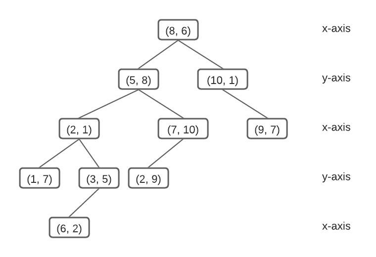
A 2-dimensional tree constructed from Ε. ~Image by author

With x as the splitting dimension for level 1, the tree compares nodes (5, 8) and (10, 1) with (8, 6) at the x-axis. As (5, 8) compares less, it branches to the left, whereas, (10, 1) branches to the right. On level 2, the assigned splitting dimension is y. The tree compares nodes (2, 1) and (7, 10) with (5, 8) at the y-axis. As (2, 1) compares less, it branches to the left, whereas, (7, 10) branches to the right.

It is easy to visualize these points in a 2d-space. The figure below shows red lines partitioning the space in x and blue lines in y dimensions.

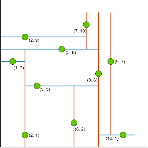
Set Ε visualized in 2d-space. ~Image by author

As you can see, the lines partition the 2d-space. Hence, called a space-partitioning algorithm.

The 2-dimensional tree makes it easier to visualize and understand the fundamental concept. Yet, the data structure applies to any number of dimensions.

In this section, we’ll focus on three fundamental operations on a kd-tree.

#machine-learning #algorithms #deep-learning #data-science #developer