In machine learning, when building a classification model with data having far more instances of one class than another, the initial default classifier is often unsatisfactory because it classifies almost every case as the majority class. Most of us are familiar with the fact that the ordinary classification accuracy score (% classified correctly) is not useful in the highly-imbalanced (skewed) case because it can trivially approach 100%, and it gives equal weight to false positives and false negatives. Many articles show you how to use oversampling (e.g. SMOTE) or sometimes class-based sample weighting to retrain the model, but this isn’t always necessary (and it also biases/distorts the numeric probability predictions of the model so that they become miscalibrated to the original and future data). Here we aim instead to show how much you can do **without **balancing the data or retraining the model, and how it gives you the flexibility to make any desired trade-off between false positives and false negatives.

We will use the credit card fraud identification data set from Kaggle to illustrate. Each row of the data set represents a credit card transaction, with the target variable Class==0 indicating a legitimate transaction and Class==1 indicating that the transaction turned out to be a fraud. There are 284,807 transactions, of which only 492 (0.173%) are frauds — very imbalanced indeed.

We will use a gradient boosting classifier because these often give good results. Specifically Scikit-Learn’s new HistGradientBoostingClassifier because it is much faster than their original GradientBoostingClassifier when the data set is relatively large like this one.

First let’s import some libraries and read in the data set.

import numpy as np
import pandas as pd
from sklearn import model_selection, metrics
from sklearn.experimental import enable_hist_gradient_boosting
from sklearn.ensemble import HistGradientBoostingClassifier
df=pd.read_csv('creditcard.csv')
df.info()

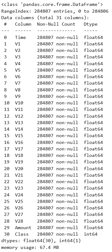
V1 through V28 (from a principal components analysis) and the transaction Amount are the features, which are all numeric and there is no missing data. Because we are only using a tree-based classifier, we don’t need to standardize or normalize the features.

We will now train the model after splitting the data into train and test sets. This took about half a minute on my laptop. We use the n_iter_no_change to stop the training early if the performance on a validation subset starts to deteriorate due to overfitting. I separately did a little bit of hyperparameter tuning to choose the learning_rate and max_leaf_nodes, but this is not the focus of the present article.

Xtrain, Xtest, ytrain, ytest = model_selection.train_test_split(
        df.loc[:,'V1':'Amount'], df.Class,  stratify=df.Class, 
        test_size=0.3, random_state=42)
gbc=HistGradientBoostingClassifier(learning_rate=0.01, 
        max_iter=2000, max_leaf_nodes=6, validation_fraction=0.2, 
        n_iter_no_change=15, random_state=42).fit(Xtrain,ytrain)

Now we apply this model to the test data as the default hard-classifier, predicting 0 or 1 for each transaction. We are implicitly applying decision threshold 0.5 to the model’s probability prediction as a soft-classifier. When the probability prediction is over 0.5 we say “1” and when it is under 0.5 we say “0”.

#imbalanced-data #classification #machine-learning #false-positive #false-negative