Motivation

Having a housing price prediction model can be a very important tool for both the seller and the buyer as it can aid them in making well informed decision. For sellers, it may help them to determine the average price at which they should put their house for sale while for buyers, it may help them find out the right average price to purchase the house.

Objective

To build a random forest regression model, which is able to predict the median value of houses. We will also briefly walk through some Exploratory Data Analysis, Feature Engineering and Hyperparameter tuning to improve the performance of our Random Forest model.

Our Machine Learning Pipeline

Our Machine Learning Pipeline can be broadly summarized into the following task:

1. Data Acquisition
2. Data Pre-Processing and Exploratory Data Analysis
3. Creating a Base Model
4. Feature Engineering
5. Hyperparameter Tuning
6. Final Model Training and Evaluation

Step 1: Data Acquisition

We will be using the Boston Housing dataset_: https://www.kaggle.com/c/boston-housing/data._

#Importing the necessary libraries we will be using

%load_ext autoreload
%autoreload 2
%matplotlib inline
from fastai.imports import *
from fastai.structured import *
from pandas_summary import DataFrameSummary
from sklearn.ensemble import RandomForestRegressor
from IPython.display import display
from sklearn import metrics
from sklearn.model_selection import RandomizedSearchCV
#Loading the Dataset
PATH = 'data/Boston Housing Dataset/'
df_raw_train = pd.read_csv(f'{PATH}train.csv',low_memory = False)
df_raw_test = pd.read_csv(f'{PATH}test.csv',low_memory = False)

Step 2: Data Pre-Processing and Exploratory Data Analysis (EDA)

2.1 Checking and handling if there are any missing data and outliers.

df_raw_train.info

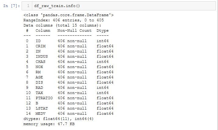
Understanding the raw data:

From the raw training dataset above:

(a) There are 14 variables (13 independent variables — Features and 1 dependent variable — Target Variable).

(b) The data types are either** integers** or floats.

© No categorical data is present.

(d) There are no missing values in our dataset.

2.2 As part of EDA, we will first try to determine the distribution of the dependent variable (MDEV).

#Plot the distribution of MEDV

plt.figure(figsize=(10, 6))
sns.distplot(df_raw_train['MEDV'],bins=30)

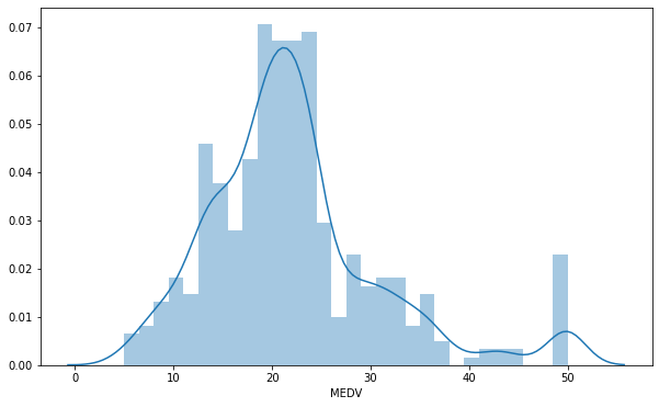
The values of MEDV follows a** normal distribution** with a mean of around 22. There are some outliers to the right.

2.3 Next, try to determine if there are any correlations between:

(i) the independent variables themselves

(ii) the independent variables and dependent variable

To do this, let’s do a correlation heatmap.

# Plot the correlation heatmap

plt.figure(figsize=(14, 8))
corr_matrix = df_raw_train.corr().round(2)
sns.heatmap(data=corr_matrix,cmap='coolwarm',annot=True)

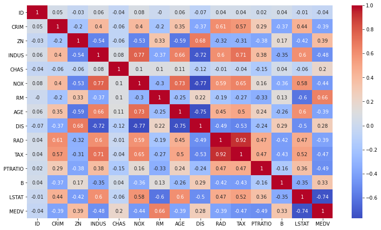
(i) Correlation between independent variables:

We would need to look out for features of multi-collinearity (i.e. features that are correlated with each other)as this will affect our relationship with the independent variable.

Observe that **RAD **and TAX are highly correlated with each other (Correlation score: 0.92) while there are a couple of features which are somewhat correlated with one another with a correlation score of around 0.70 (INDUS and TAX, NOX and INDUS, AGE and DIS, AGE and INDUS).

(ii) Correlation between independent variable and dependent variable:

In order for our regression model to perform well, we ideally need to select those features that are highly correlated with our dependent variable (MEDV).

We observe that both RM and LSTAT are** correlated** with MEDV with a correlation score of 0.66 and 0.74 respective. This can also be illustrated via the scatter plot .

#sklearn #random-forest #boston #data-science #data analysis