In the previous post, we presented the Value-based Agents and reviewed the Bellman equation one of the central elements of many Reinforcement Learning algorithms. In this post, we will present the Value Iteration method to calculate those V-values and Q-values required by Value-based Agents.

Calculating the V-value with loops

In the simple example presented in the previous post, we had no loops in transitions and was clear how to calculate the values of the states: we could start from terminal states, calculate their values, and then proceed to the central state. However, only the presence of a loop in the environment prevents this proposed approach.Let’s see how these cases are solved with a simple Environment with two states, state 1 and state 2, that presents the following environment’s states transition diagram:

We only have two possible transitions: from state 1 we can take only an action that leads us to state 2 with Reward +1 and from state 2 we can take only an action that returns us to the state 1 with a Reward +2. So, our Agent’s life moves in an infinite sequence of states due to the infinite loop between the two states. What is the value of both states?Suppose that we have a discount factor γ<1, let’s say 0,9, and remember from the previous post that the optimal value of the state is equal to that of the action that gives us the maximum possible expected immediate reward, plus the discounted long-term reward for the next state:

In our example, since there is only one action available in each state, our Agent has no other option and therefore we can simplify the previous formula as:

For instance, if we start from state 1, the sequence of states will be [1,2,1,2,1,2, …], and since every transition from state 1 to state 2 gives us a Reward of +1 and every back transition gives us a Reward of +2 the sequence of Rewards will be [+1,+2,+1,+2,+1,+2, …]. Therefore, the previous formula for state 1 becomes:

Strictly speaking, it is impossible to calculate the exact value of our state, but with a discount factor γ= 0,9, the contribution of a new action decreases over time. For example, for the sweep i=37 the result of the formula is 14.7307838, for the sweep i=50 the result is 14.7365250 and for the sweep i=100 the result is 14.7368420. That means that we can stop the calculation at some point (e.g. at i=50) and still get a good estimate of the V-value, in this case V(1) = 14.736.

The Value Iteration Algorithm

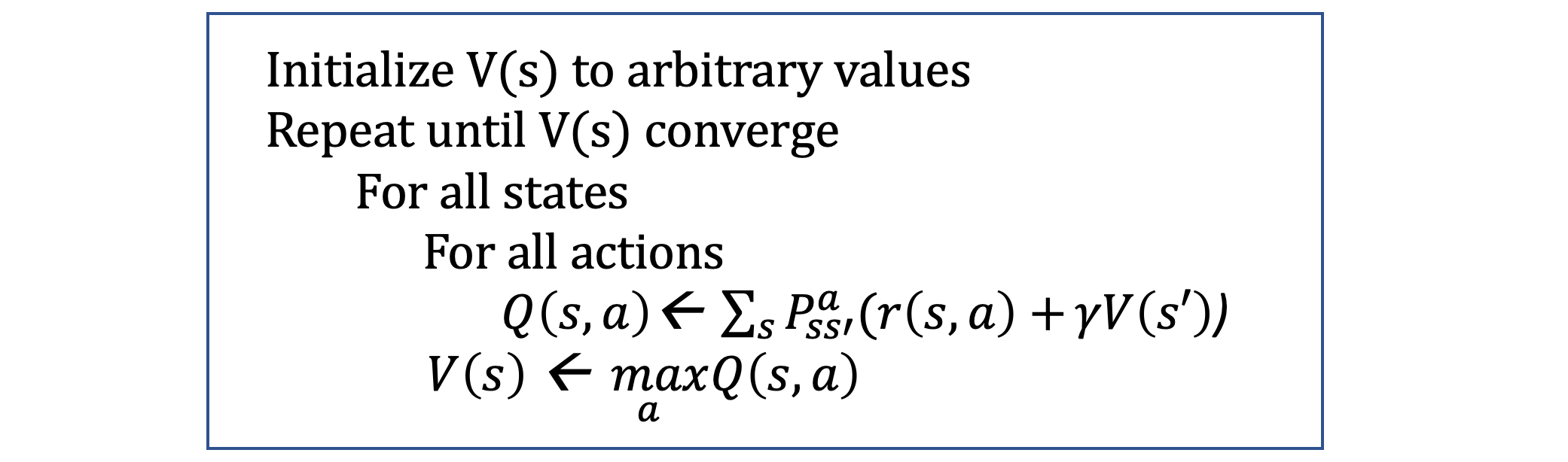
The preceding example can be used to get the gist of a more general procedure called the** Value Iteration algorithm (VI)**. This allows us to numerically calculate the values of the states of Markov decision processes, with known transition probabilities and rewards.The idea behind the Value Iteration algorithm is to merge a truncated policy evaluation step (as shown in the previous example) and a policy improvement into the same algorithm.Basically, the Value Iteration algorithm computes the optimal state value function by iteratively improving the estimate of V(s). The algorithm initializes V(s) to arbitrary random values. It repeatedly updates the Q(s, a) and V(s) values until they converge. Value Iteration is guaranteed to converge to the optimal values. The following pseudo-code express this proposed algorithm:

Estimation of Transitions and Rewards

In practice, this Value Iteration method has several limitations. First of all, the state space should be discrete and small enough to perform multiple iterations over all states. This is not an issue for for our Frozen-Lake Environment but in a general Reinforcement Learning problem, this is not the case. We will address this issue in subsequent posts in this series.Another essential practical problem arises from the fact that to update the Bellman equation, the algorithm requires knowing the probability of the transitions and the Reward for every transition of the Environment.Remember that in our Frozen-Lake example, we observe the state, decide on an action, and only then do we get the next observation and reward for the transition but we don’t know this information in advance. What can we do to get them?Luckily, what we can have is the history of the Agent’s interaction with the Environment. So, the answer to the previous question is to use our Agent’s experience as an estimation for both unknowns. Let’s see below how we can achieve it.

Estimation of Rewards

Estimate Rewards is the easiest part since Rewards could be used as they are. We just need to remember what reward we got on the transition from s to s’ using action a.

Estimation of Transitions

To estimate transitions is also easy, for instance by maintaining counters for every tuple in the Agent’s experience(s, a, s’) and normalize them.For instance, we can create a simple table that keeps the counters of the experienced transitions. The key of the table can be a composite “state” + “action”, (s, a), and the values of each entry there is the information about target states, _s’, _and a count of times that we have seen each target state, c.Let’s look at an example. Imagine that during Agent’s experience, in a given state s0 it has executed an action a several times and it ends up c1 times in state s1 and c2 times in state s2. How many times we have switched to each of these states is stored in our transition table. That is, the entry (s,a) in the table contents {s1: c1, s2: c2}. Perhaps visually you can more easily see the information contained in the table for this example:

Then, it is easy to use this table to estimate the probabilities of our transitions. The probability that the action will take us from state 0 to state 1 is c1 / (c1 + c2) and that the action will take us from state 0 to state 2 c2 / (c1 + c2).

#machine-learning #data-science #algorithms