Comparing what you see during an eclipse to the darkness at night is like comparing an ocean to a teardrop. ~Wendy Mass

Wendy presumably suggested that the lucidity of sight during an eclipse in dimness is generously more clear than an ordinary night. Or maybe a normal night isn’t anything when contrasted with the obscurity during a shroud. Similarly, I feel Time-series ideas stay in obscurity until Maths make it more understood. Even though the recurrence of using legitimate Maths in routine is practically similar to an obscuration, yet the intensity of clarifying Time-series through mathematical proofs isn’t anything when contrasted with utilizing a measurable statistical tool to fight and envision some information. However, I wish to engage my readers with the “teardrop” today before they take a plunge into the ocean. The explanation being each night has the Moon, and strolling in the evening glow is precisely sentimental until science hands over some light to see through. The motivation behind this article is to see a tad bit of Time-series precisely through various tools (simply like each night) expecting the obscuration of numerical clarifications is uncommon and distant yet unquestionably important to take a gander at the sky in another manner.

Agenda

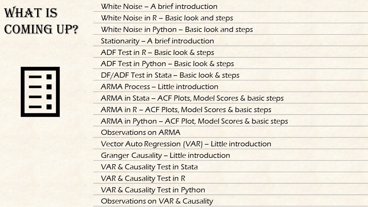
Article Agenda, Image Source : (Image from Author)

White Noise

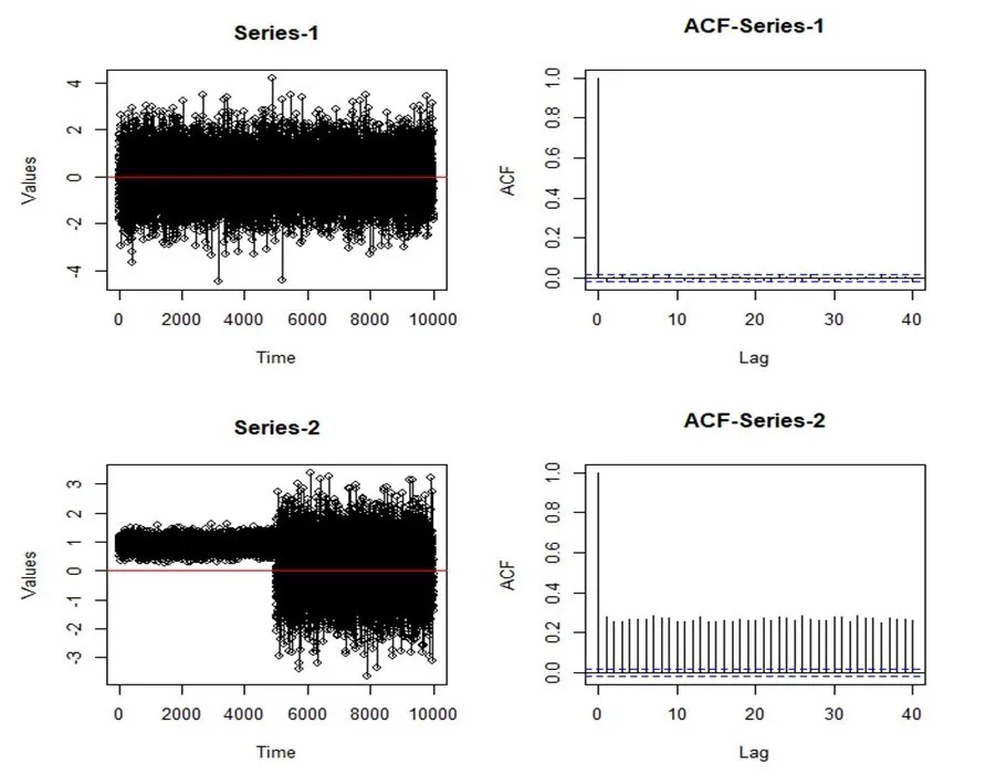
In literary terms, white noise is the sound produced by all frequencies of sound together at once. It can be heard and we must have heard one way or the other. Here is a link if we haven’t. In our case white noise is a time series that satisfies **three **conditions; a series with zero mean, constant variance, and no correlation between two consecutive elements of the series. A white noise series is not predictable and hence an indication that it does not require any analysis further. To test the third condition we generally use an ACF (autocorrelation function) plot, which tests the correlation between two consecutive observations. If the correlation is non zero then the bars at that lag would **cross **the boundary lines on each side.

R View

The first series has an approximate zero mean and 1 variance, whereas the second series has an approximate mean of 0.5 and 0.7 variance. The ACF plot has no bands crossing the threshold boundary except 0th lag (which is the correlation of the observation with itself). The ACF plot of the second series has outright lagged correlations. Visually too, we can verify the variations change in the second series.

#timeseries #data-science #analytics