To perform Linear Regression, Data should accomplish the below constraints:

1. Data should be Continuous.
2. There should be a Correlation & Causation exists between Independent & Dependent Variable.

To research deeper into the concept of why Regression made on Continuous and Correlated data, please check this page.

If the Linear Regression is made on one independent variable, plotting of data will be similar to the below scatter plot.

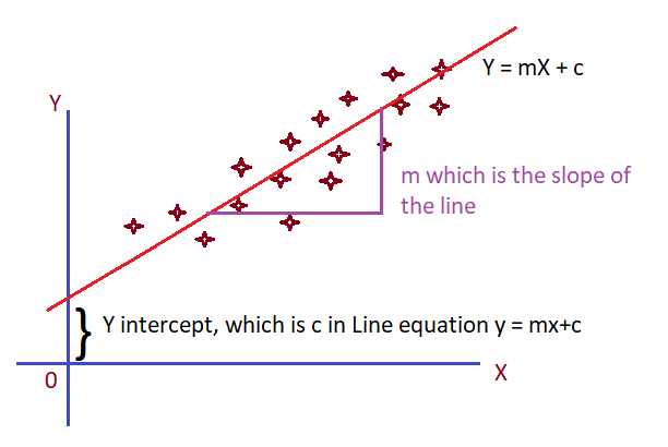
Linear Regression

X — Independent Variable i.e. Input training data

Y — Dependent Variable, i.e. Output data

In mathematical way, every line has an equation. Y = mX + c

For a straight line the m & c value will be constant and X is a set of values.

slope = m = rise/run = dy/dx i.e. Change in Y/Change in X

For example, if (m, c) is (2,1) then the equation becomes Y = 2X + 1

In the above example linear regression model, as the data is in a good correlation, a line can be drawn such that it runs in a way that all the points in the graph is most possibly near to the line, which is called a line of best fit. Thus, we can be sure that for any new value of X, the Y value is where the perpendicular line from X point meets the Straight line.

Let ŷi is the Y value as predicted by the line of regression when x = xi.

Then for each point there is an error/difference between the predicted and actual value which can be defined as Ei = yi — ŷi.

As an overall error, we need to find this difference for all the existing input data and sum its square (SSE)which we will see in this article (Section Cost Function).

#regression #linear-regression #cost-function