Logistic regression is the first non-linear function that undergraduate statistics students learn to use. It is also the first classification algorithm that MOOCs teach to aspiring data scientists.
There are a few reasons why logistic regression is so popular:
- It is easy to understand.
- It only requires a few lines of code.
- It is a great introduction to binary response models.
In this article, I will explain the math behind the logistic regression, including how to interpret the coefficients of the logistic regression model, and explain the advantages of logistic regression over a more _naive _method.
This is part one of a two-part series on logistic regression. In part two, we will build a logistic regression model in Python.
A Primer on Estimating Probabilities with Regression
Before delving into logistic regression, let’s first discuss a simpler, though intuitively similar, model:
Linear Probability Model (LPM).
The Linear Probability Model is identical to a regression model except for a key difference:
whereas the dependent variable for a regression model is continuous, the dependent variable for a LPM is binary.
If we have one independent variable, then our LPM is
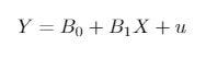
Image by author
where Y is a binary response variable, _X _is an independent variable, and _u _is the error term.
For every one-unit change in X, the probability that _Y _equals 1 changes by B1. If _X _equals 0, then the probability that _Y _equals 1 is B0.
Let’s use a practical example. Suppose that Y equals 1 if a person is employed, and 0 if they are not. _X _is their years of post-secondary education.
#data-science #statistics #machine-learning #regression #deep-learning