“Computers are able to see, hear and learn. Welcome to the future” — Dave Walters

It has been well established and documented that the computational capabilities of computers far exceed that of human beings. Hence, since the middle of the 20th century, computation heavy activities have been attempted to be gradually automated by leveraging computers. With the advent and increasing proficiency of application of Machine Learning (ML), predictive models have taken precedence. Some of the examples of where ML has taken over are

1. Customer retention by proactive identification of customers likely to terminate subscription
2. Forecasting of sales, demand, revenue etc. for any industry
3. Identification of customers for cross-selling, in any industry
4. Identification of customers likely to default in let’s say mortgage payments
5. Preventive Maintenance of machines by identification of machines likely to break down

However problems that had historically required human perception for arriving at the solution, were beyond the reach of classical (static) ML algorithms. The good news is that with the massive break throughs in Deep Learning (DL) since early 2010s, near human-like performance is being observed in solving such problems that traditionally required human intuition. The aforementioned perceptual problems required skills to process sound and images. So the ability to sense and process, through hearing and seeing seemed to be the major skill that could facilitate solution of such problems. These skills came naturally and intuitively to humans but had been long elusive for machines. Some of the examples of perceptual problems solved through application of DL are given below

• Near-human-level image classification and object detection
• Near-human-level speech recognition
• Near-human-level handwriting transcription
• Improved machine translation
• Improved text-to-speech conversion
• Digital assistants such as Google Now and Amazon Alexa
• Near-human-level autonomous driving
• Ability to answer natural-language questions

It must however be said that, this is just the beginning and we are merely scratching the surface of what can be achieved. There is research going on to foray into the space of formal reasoning as well. If successful, this may help human beings in fields of science, psychology, software development etc.

The question that comes to mind is, how does the machine do this i.e. gain the perceptual power to solve problems requiring human intuition. Number crunching, solving problems dealing with numbers and/or categories, with the application of supervised learning (or unsupervised learning) was within the realms of machines with huge computational capabilities. Being able to see and recognize components of an image is a new skill and this article’s focus is to bring to attention the process that is now giving computers the ability to see and perform like humans in solving problems involving images. The content for this article includes the following

1. A brief introduction to Artificial Intelligence (AI) and Deep Learning (DL)
2. Image Recognition by application of Fully Connected Layers (FCN) i.e. Multi-layer perceptron’s (MLP)
3. Introduction to Convolution Neural Networks (CNN)
4. Why is CNN used over MLPs for solving Image related problems
5. Working of a CNN
6. Comparison of performance between MLP and CNN

A brief introduction to Artificial Intelligence (AI) and DL

AI is a field that enables computers to mimic human intelligence by application of logic, if-then rules, decision trees and ML (including DL). Artificial Neural Network (ANN) is a branch of AI. The below pictorial representation will further elucidate the subsets of AI i.e. ML and DL. Data Science cuts across all layers of AI.

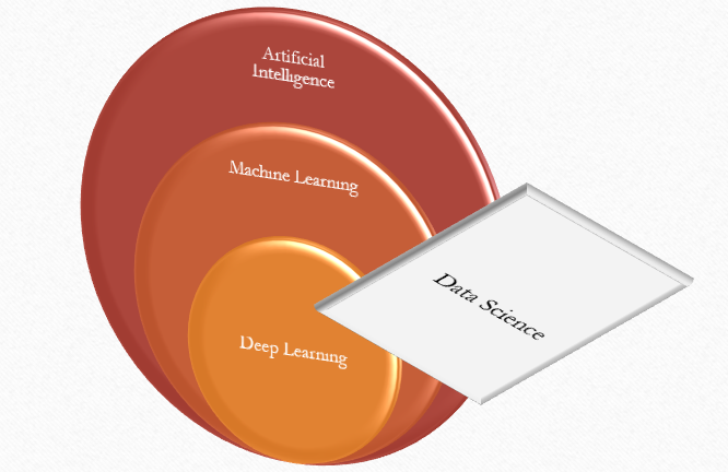
Figure 1: Subsets of AI

The foundations of any ANN architecture starts with the premise that, the model needs to go through multiple iterations making allowance for mistakes, learn from mistakes and achieve salvation or saturation when it has learnt enough, thereby producing results equal to or similar to reality. The picture below gives us a brief idea of how an ANN looks like and introduce DL Neural Network.

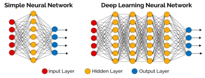
Figure 2: Comparison of a Shallow network with a DLNN (Image from an earlier article of the author)

ANN essentially is a structure consisting of multiple layers of processing units (i.e. neurons) that take input data and process it through successive layers to derive meaningful representations. The word deep in Deep Learning stands for this idea of successive layers of representation. How many layers contribute to a model of the data is called the depth of the model. The above diagram illustrates the structure better as we have a simple ANN with only one hidden layer and a DL Neural Network (DNN) with multiple hidden layers. Thus DL or DLNN is an ANN with multiple hidden layers.

The readers of this article are assumed to be familiar with the concepts that constitute the foundations of Supervised Learning and how DL leverages it to learn the patterns in data (in this case patterns in image) for achieving accurate results. Conceptual understanding of the below items will be required for better understanding of the rest of the article

• Supervised Learning
• Deep Learning
• Loss Function
• Gradient Descent
• Forward and Backward Propagation

For refresher, the reader can explore freely available material on these topics in internet or go through my published article, Foundations of Deep Learning. Going through each of the above concepts in-depth is beyond the scope of this article.

Image Recognition by application of Fully Connected Layers i.e. Multi-layer Perceptron’s

Let’s now delve into an practical example of how an ANN can be leveraged to see images and classify them to appropriate categories. We will start with application of a FCN on a real world dataset and gauge the efficiency achieved. The reader is assumed to have deeper understanding of what is a FCN and how it operates. At a very high level, FCN or MLP is an ANN where each element of every layer is connected to each element of the following layer. Figure 3 below illustrates how a FCN looks like. For more details, please refer to my published article, Foundations of Deep Learning.

The problem we will try to solve involves recognition of digits from images of house numbers taken from streets. The data set name is Street View House Numbers (SVHN). SVHN is a real-world image dataset for developing machine learning and object recognition algorithms with minimal requirement on data formatting but comes from a significantly harder, unsolved, real world problem (recognizing digits and numbers in natural scene images). SVHN is obtained from house numbers in Google Street View images.

The goal we are going to achieve is to take an image from the SVHN dataset and determine what that digit is. This is a multi-class classification problem with 10 possible classes, one for each digit 0–9. Digit ‘1’ has label 1, ‘9’ has label 9 and ‘0’ has label 10. Although, there are close to 6,00,000 images in this dataset, we have extracted 60,000 images (42000 training and 18000 test images) to do this project. The data comes in a MNIST-like format of 32-by-32 RGB images centered around a single digit (many of the images do contain some distractors at the sides).

We will use raw pixel values as input to the network. The images are matrices of size 32×32. So, we reshape the image matrix to an array of size 1024 ( 32*32 ) and feed this array to a ANN like below.

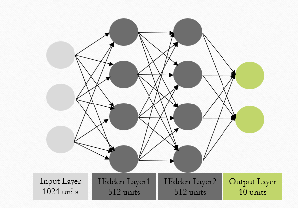
Figure 3: FCN Architecture

Link to the dataset is here.

Below are the codes to load the data and visualize a few of the images.

## Import the data
import h5py
import numpy as np

ds=h5py.File('/content/drive/My Drive/--/SVHN_single_grey1.h5','r')

X_train = ds['X_train'][:]
y_train = ds['y_train'][:]
X_test = ds['X_test'][:]
y_test = ds['y_test'][:]

## Close this file
ds.close()
## visualizing the data
plt.imshow(X_train[0])
plt.axis('off')

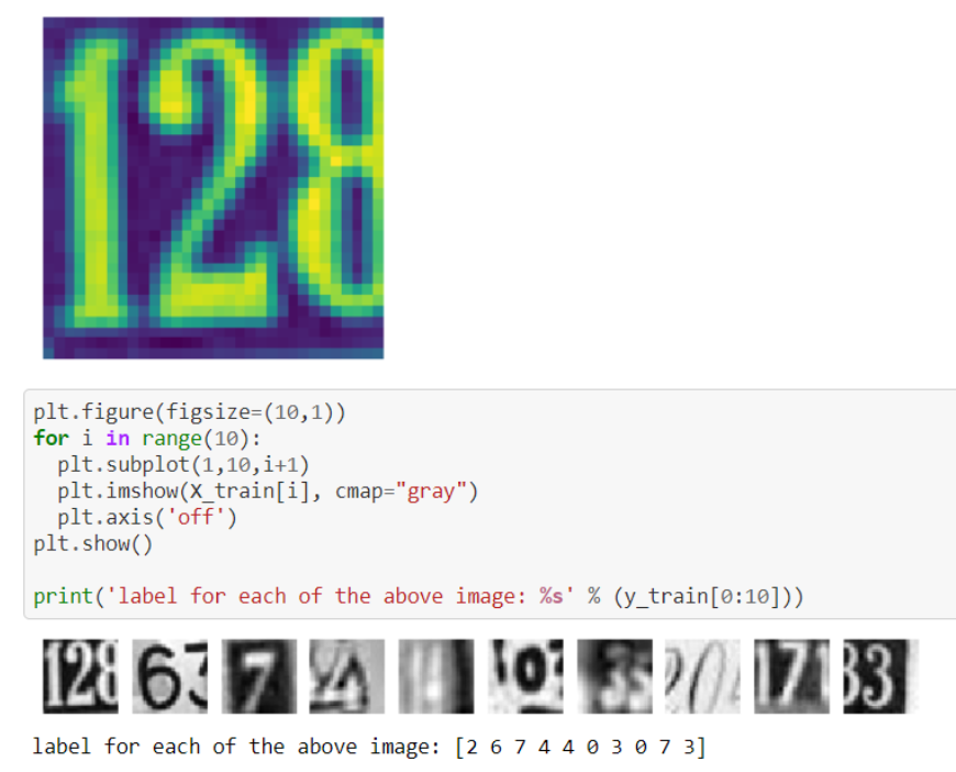
Figure 4: Screenshot from Jupyter notebook for display of a few images and their labels

Multiple MLPs were built with different number of hidden layers and different number of neurons in each of the layers. The results from each model was compared and the best was achieved with three hidden layers. The model architecture is given below. It achieved an accuracy of ~80%.

def mlp_model():
    model = Sequential()

    model.add(Dense(248*4, input_shape = (1024, ), kernel_initializer='he_normal'))
    model.add(BatchNormalization())
    model.add(Activation('relu'))
    model.add(Dropout(0.5))
    model.add(Dense(248*4, kernel_initializer='he_normal'))
    model.add(BatchNormalization())
    model.add(Activation('relu')) 
    model.add(Dropout(0.5))
    model.add(Dense(248*4, kernel_initializer='he_normal'))
    model.add(BatchNormalization())
    model.add(Activation('relu')) 
    model.add(Dropout(0.5))
    model.add(Dense(248*4, kernel_initializer='he_normal'))
    model.add(BatchNormalization())
    model.add(Activation('relu'))    
    model.add(Dropout(0.5))
    model.add(Dense(10, kernel_initializer='he_normal'))
    model.add(Activation('softmax'))

    adam = optimizers.adam(lr = 0.0001)
    model.compile(optimizer = adam, loss = 'categorical_crossentropy', metrics = ['accuracy'])

    return model

model = mlp_model()
history = model.fit(X_train, y_train,batch_size=2048 ,epochs = 200, verbose = 1, validation_data=(X_test, y_test))

The visualization of how the loss gradually decreased and accuracy increased iteratively is depicted below

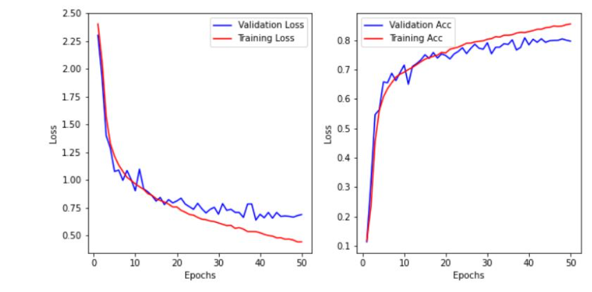
Figure 5: Screenshot from Jupyter Notebook

A few of the images in the test data (which was not exposed to the training process) were predicted. Visualization for the same and comparison with it’s original label is given below.

import numpy as np

plt.figure(figsize=(2,2))
plt.imshow(X_test[50])
plt.show()
print( "Actual Digit is: ",np.argmax(m.predict(test_X)[50]))

plt.figure(figsize=(2,2))
plt.imshow(X_test[500])
plt.show()
print( "Actual Digit is: ",np.argmax(m.predict(test_X)[500]))

plt.figure(figsize=(2,2))
plt.imshow(X_test[1500])
plt.show()
print( "Actual Digit is: ",np.argmax(m.predict(test_X)[1500]))

#deep-learning #artificial-intelligence #opencv #developer