In this article, I will summarize my short experience with Super-Resolution task based on the PASCAL-VOC 2007 data set. During this session, I have tried several different models for super resolution of images from size of 72723 to 1441443 and to 2882883.

First thing needed for this task is getting the data set, I used the Kaggle

preloaded data set.

Because I trained different models and had a lot of data, for this entire work I used data generator for loading the images and for resizing them.

Data generator for loading images

import cv2
import os

image_dir = '../input/pascal-voc-2007/voctrainval_06-nov-2007/VOCdevkit/VOC2007/JPEGImages'
def load_images_iter(amount = 64,start_pos = 0, end_pos = 5011):
  ans = []
  all_im = os.listdir(image_dir)
  all_im.sort()
  print (len(all_im))
  while (True):
    for idx,img_path in enumerate(all_im[start_pos:end_pos]):
      if (len(ans) !=0 and len(ans)%amount == 0):
        ret = ans
        ans = []
        yield ret
      ans.append(cv2.imread(image_dir+"/"+img_path))

The sort function here isn’t mandatory. I used it because I use the generators not only for training and validating the model but also for looking at the model results. Therefore, I need to make sure I look at the same pictures all the time, So the sort function guarantees that.

I’ve created several different generators for the different uses. here is an example of a generator for the training set (the data was split that first 1000 pictures are for validation and the rest for training).

For resizing the images I used CV2 resize function.

Data Generator for Train

the generator returns a tuple, the first value is the train and the second value is another tuple of the output21 and output 2 expected results.

def train_generator_2(batch=64, tar1_size=144, tar2_size=288 , train_size=72):
  collect_train = []
  collect_target_1 = []
  collect_target_2 = []
  while True:
      file_gen = load_images_iter(amount=batch, start_pos = 
                          1000)#first 1000 images are for validation
      imgs = []
      while (True):
        try:
          imgs = next(file_gen)
        except:
          break
        for idx,img in enumerate(imgs): 
          if (len(collect_train)!=0 and
                  len(collect_train)%batch == 0):
            ans_train = np.asarray(collect_train,dtype=np.float)
            ans_target_1 = 
              np.asarray(collect_target_1,dtype=np.float)
            ans_target_2 = 
              np.asarray(collect_target_2,dtype=np.float)
            collect_train = []
            collect_target_1 = []
            collect_target_2 = []
            yield (ans_train, (ans_target_1,ans_target_2))
          collect_train.append(cv2.resize(img,
                              (train_size,train_size))/255.0)
          collect_target_1.append(cv2.resize(img,
                                 (tar1_size,tar1_size))/255.0)
          collect_target_2.append(cv2.resize(img,
                                 (tar2_size,tar2_size))/255.0)

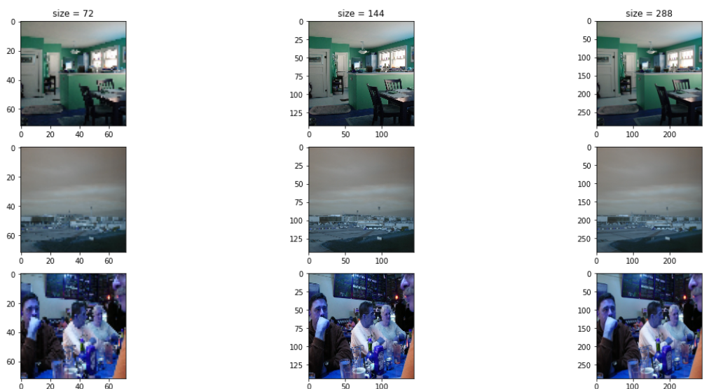
As with any machine learning and deep learning jobs, I started with some data exploration.

We have 5011 different pictures with different sizes. The Pictures have no common motive between them, or any noticeable similarity . Here are some sample pictures In different sizes:

For all the models in this assignment I used MSE as the loss function and PSNR as the metric.

The model’s loss was combined from the 2 outputs loss evenly. And each output had its own PSNR metric.

from keras import backend as K
import math

def PSNR(y_true, y_pred):
    max_pixel = 1.0
    return 10.0 * (1.0 / math.log(10)) * K.log((max_pixel ** 2) / (K.mean(K.square(y_pred - y_true))))

First Model

So the first model I’ll discuss is a basic model with 2 outputs for 2 different size images (1441443, 2882883).

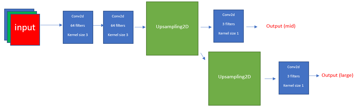
First Model Structure

From this structure, we can see that in order to get the required size we need to keep the original input height and width dimensions. So for the convolutional layers, I used padding.

inp = Input((72,72,3))
x = Conv2D(64,(3,3), activation = 'relu', padding = 'same')(inp)
x = Conv2D(64,(3,3), activation = 'relu', padding = 'same')(x)
x = UpSampling2D(size=(2,2))(x)
x = Conv2D(3,(1,1), activation = 'relu', padding = 'same')(x)

model1 = Model(inputs = inp ,outputs = x)

First Model Loss

This model is pretty simple thus starts to converge pretty quickly as can be seen in the graph.

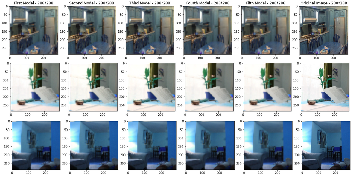
So In first sight, it seems we get pretty good results from the loss function but if we will take an actual look at the images they tell a different story.

In the picture below:

The 2 images on the right are the images downsized to sizes 144144, and 288288.

The 2 images on the left are the model predictions with respective sizes.

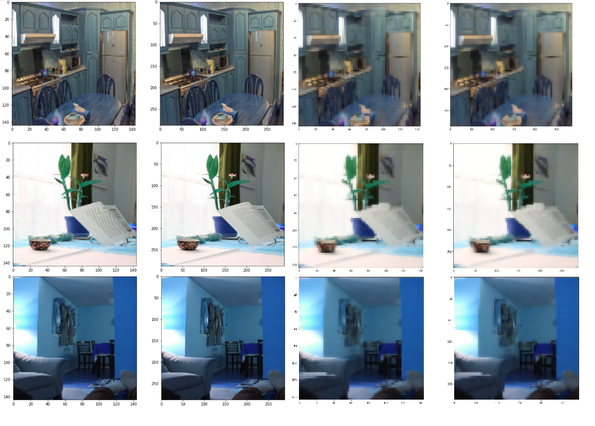
Downsized Images VS First Model Predictions

We can see here that although the loss is good we still actually get pretty bad results.

First Model PSNR Graph

If we take a look at the PSNR graph we see it converges around the 21 which apparently isn’t such a good result. Also, we need to keep in mind that high PSNR doesn’t assure an image that looks good to the human eye, this is only an auxiliary metric to help us understand a little bit better how good or bad is the model.

Second Model

In this model, I tried to residual blocks instead of the convolutional layers.

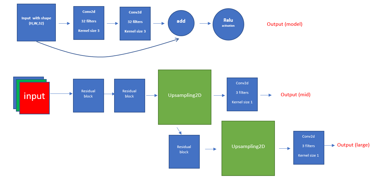
Model Structure

This model structure added more parameters to our model, so maybe it will help us improve the results we get.

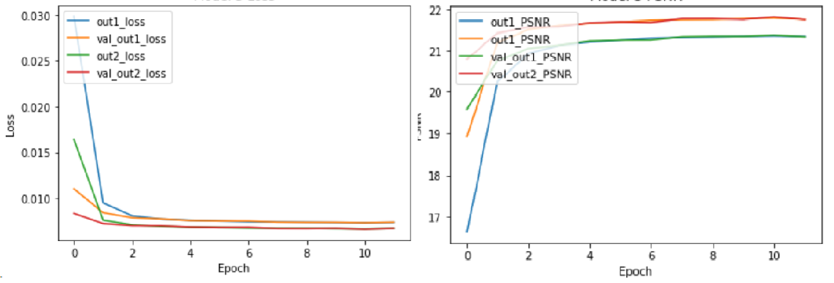
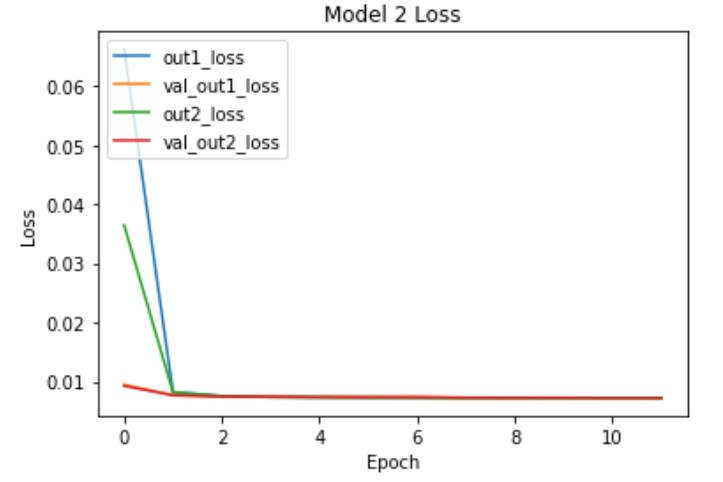
Second Model Loss & PSNR graphs

Here we can see that we get convergence after 2 epochs just as before, the loss is a tiny bit better and also the PSNR. But will this mean we also have better images?

#deep-learning #super-resolution #deep learning