In my previous blog post we worked on artificial neural networks and developed a class to build networks with arbitrary numbers of layers and neurons. While the blog referenced to the previous notebook explaining the prerequisites, there was not yet the accompanying article, which is this blog post.
This post is also available as a Jupyter Notebook on my Github, so you can code along while reading.
If you are new to Python and Jupyter, here is a short explanation on how I manage my Python environment and packages.
A short overview of the topics we will be discussing:
- Link between neural networks and logistic regression
- One step back: linear regression
- From linear to (binary) logistic regression
- Round up
Link between neural network and logistic regression
When we hear or read about deep learning we generally mean the sub-field of machine learning using artificial neural networks (ANN). These computing systems are quite successful in solving complex problems in various fields, examples are, image recognition, language modelling, and speech recognition. While the name ANN implies that they are related to the inner workings of our brain, the truth is that they mainly share some terminology. An ANN generally consists of multiple interconnected layers, which on itself are build using neurons (also called nodes). An example is shown in figure 1.
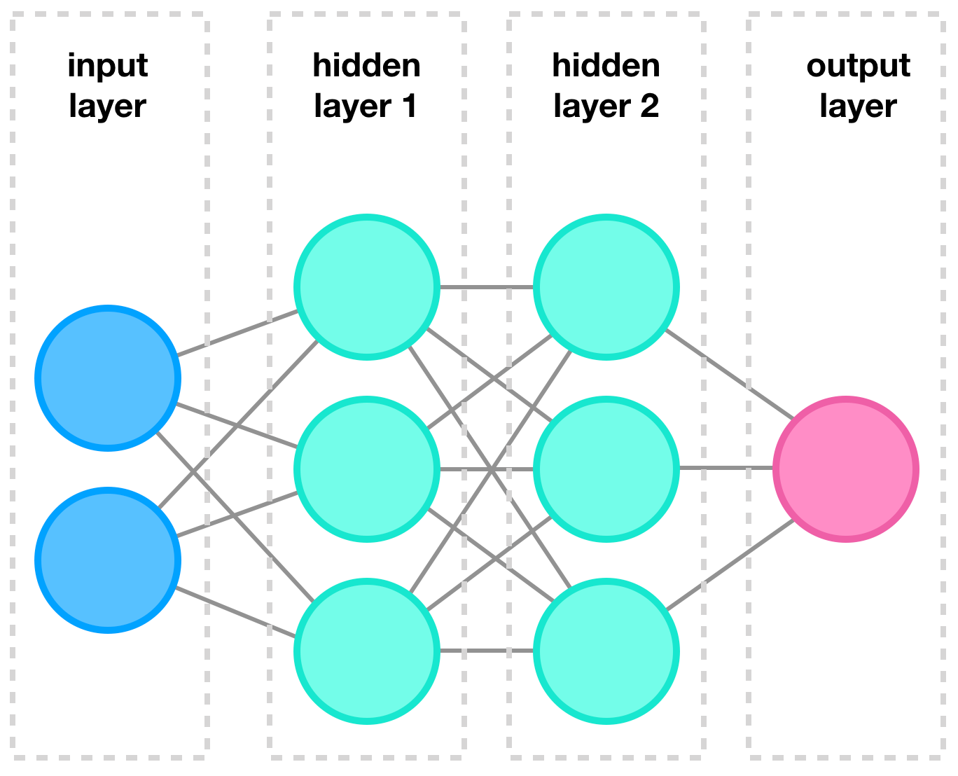
Figure 1: Example of a typical neural network, borrowed from my follow up article on neural networks.
In this example, we have one input layer, consisting of four individual inputs nodes. This input layer is ‘fully connected’ to the first hidden layer, i.e. Fully connected means that each input is connected to each node. The first hidden layer is again fully connected to another ‘hidden’ layer. The term hidden indicates that we are not directly interact with these layers and these are kind of obscured to the user. The second hidden layer is on its turn fully connected two the final output layer, which consists of two nodes. So in this example we feed the model four inputs and we will receive two outputs.
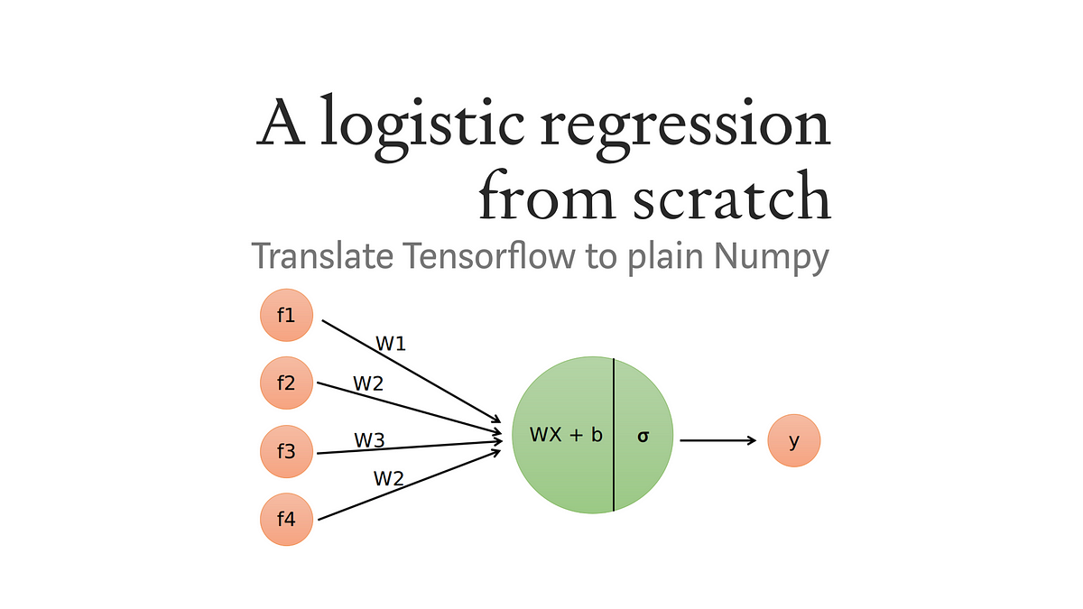
Let’s now focus on a single neuron from our previous example. This neuron still is connected to all inputs, also called features. Using these features, the neuron calculates a single response (or output). A diagram of such a system is depicted in figure 2.
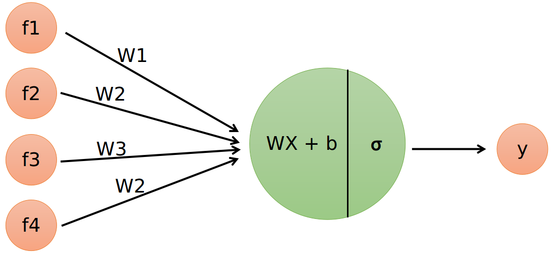
Figure 2: single neuron with four input features. The neuron has two operations: a linear part and the activation function.
The input features are named 𝑓¹, 𝑓², 𝑓³, and 𝑓⁴ and are all connected to the single neuron. This neuron executes two operations. The first operation is a multiplication of the features with a weight vector 𝑊 and adding the bias term 𝑏. The second operation is a so called activation function, indicated here by 𝜎. The output of the neuron is a probability between zero and one. The single neuron acts like a small logistic regression model and therefore, an ANN can be seen as a bunch of interconnected logistic regression models stacked together. While this idea is pretty neat, the underlying truth is a bit more subtle. There are many different architectures for ANNs and they can use various building blocks that act quite different than in this example.
The linear operation in our single neuron is nothing more than a linear regression. Therefore, to understand logistic regression, the first step is to have an idea how linear regression works. The next section will show a step by step example as a recap.
One step back: linear regression
What is a linear regression again?
Linear regression in its simplest form (also called simple linear regression), models a single dependent variable _𝑦 _using a single independent variable 𝑥. This may sound daunting, but was this means is that we want to solve the following equation:
𝑦 = a𝑥 + 𝑏
In the context of machine learning, 𝑥 represents our input data, 𝑦 represents our output data, and by solving we mean to find the best weights (or parameters), represented by 𝑤 and 𝑏 in the linear regression equation. A computer can help us find the best values for 𝑤 and 𝑏, to have the closest match for 𝑦 using the input variable 𝑥.
For the next examples, let us define the following values for x and y:
𝑥 = [−2,−1,0,1,2,3,4,5]
𝑦 = [−3,−1,1,3,5,7,9,11]
The values for 𝑥 and _𝑦 _have a linear relation so we can use linear regression to find (or fit) the best weights and solve the problem. Maybe, by staring long enough at these values, we can discover the relation, however it is much easier to use a computer to find the answer.
If you have stared long enough or just want to know the answer, the relation between _𝑥 _and 𝑦 is the following:
𝑦 = 2𝑥 + 1
In the next section we will use Tensorflow to create our single neuron model and try to ‘solve’ the equation.
#machine-learning #data-science #neural-networks #data analysis