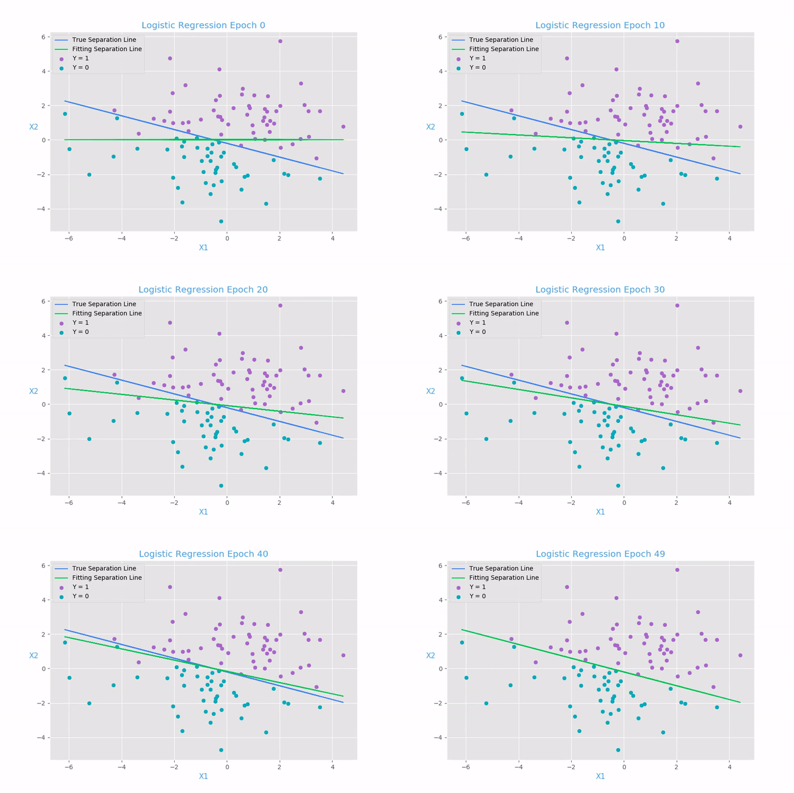
What is Logistic Regression?

Logistic Regression is one of the basic and popular algorithms to solve a classification problem, unlike its name which has Regression in it. It is named as ‘Logistic Regression’, because its underlying technique is quite the same as Linear Regression. One of the logistic regression’s advantages is because it can handle various types of relationships, not limited to linear relationships.

Let’s try to understand the Geometric Intuition behind Logistic Regression:

There is more than one approach to understanding logistic regression majorly as Probabilistic Approach, Geometric Approach, and Loss function Minimisation approach, but among all Geometric Approach is what I personally feel is more intuitive to understand. So let’s see :

Assumptions: The underlying assumption for the Logistic Regression is that data is almost or perfectly linearly separable i.e either all (+ve) and (-ve) classes are separated and if not, very few of them are mixed.

Objective: Our objective is to find a plane (**π) **That best separates (+ve) and (-ve) classes.

**Basics: **Let’s have a look at some of the basic terminologies that will make things easier to understand.

We will represent a plane with. Pi(𝜋) and Normal to Plane with** W**

Equation of plane :

Plane Visualisation

w^t*xi+b=0, where b is scalar and xi is the ith observation. and If the plane passes through origin the equation becomes w^t*xi = 0,

Where w^t(read as Wtranspose) is row vector and **xi **is a column vector

Geometric Interpretation :

Plane separating +ve and -ve classes

If we take any +ve class points, their distance di from the plane is computed as :

(di = w^t*xi/||w||. let, norm vector (||w||) is 1)

Since w and xi in the same side of the decision boundary then distance will be +ve. Now compute dj = w^t*xj since xj is the opposite side of w then distance will be -ve.

we can easily classify the point into -ve and +ve points by using if (w^tx >0) then +ve class and if (w^tx <0) then -ve class

So our classifier is :

If w^t * xi > 0  :  then Y = +1    where Y is the class label
If w^t * xi < 0  :  then Y = -1    where Y is the class label

Observations :

Carefully looking at the points on the above diagram we observe the following cases:

case 1: Yi >0 and  w^t * xi > 0
Yi = +1 means that the correct class label is +ve => Yi* w^t * xi >0 means that we have correctly predicted the class label.
as +ve * +ve = +ve

case 2: Yi <0 and  w^t * xi <0
Yi = -1 means that the correct class label is -ve => Yi* w^t * xi >0 means that we have correctly predicted the class label.
as -ve * -ve = +ve
case 3: Yi >0 and  w^t * xi <0
Yi = +1 means that the correct class label is -ve => Yi* w^t * xi <0 means that we have wrongly predicted the class label.
as +ve * -ve = -ve 
case 2: Yi <0 and  w^t * xi >0
Yi = -1 means that the correct class label is -ve => Yi* w^t * xi <0 means that we have wrongly predicted the class label.
as -ve * +ve = -ve 

#algorithms #data-science #logistic-regression #classification-algorithms #machine-learning #algorithms