Overview

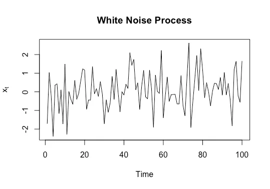
In brief, stationarity is a condition that shows whether the data has a constant mean and variance in each location. Stationarity is widely used in time series function, nevertheless we also need to know its application in terms of spatial data estimation.

There are 2 important things quoted from one of the Michael Pyrcz lecture courses:

1. Stationarity is a decision, not an hypothesis; therefore it cannot be tested. Data may demonstrate that it is inappropriate.
2. The stationarity assessment depends on scale. This choice of modeling scale(s) should be based on the specific problem and project needs.

To investigate/assess stationarity in spatial data, practically we can use two ways of visualizations, either by using a **trend plot **or a variogram plot.

Case Study — Python Codes

let’s say in “X” field , we have a Silver (Ag) distribution as follows.

import pandas as pd

df = pd.read_csv(‘contoh.csv’)
df = df[[‘ID’,’XCOO’,’YCOO’,’Ag’]]

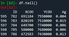
Figure 1. Ag percentage distribution data

ID is the identifier of each sample taken from the field, while XCOO and YCOO are X and Y coordinates respectively. To recognize the variation of our data, we visualize it in ID vs AG plot using pyplot as figure 2 below:

import matplotlib.pyplot as plt

plt.figure()
plt.plot(df.ID,df.Ag,color=’k’)
plt.title(‘Ag Field Data’)
plt.xlabel(‘ID’)
plt.ylabel(‘Ag’)
plt.show()

#artificial-intelligence #machine-learning #spatial-analysis #data-analytics #python