Part 3 of the tutorial series on how to implement a YOLO v3 object detector from scratch in PyTorch.

This is Part 3 of the tutorial on implementing a YOLO v3 detector from scratch. In the last part, we implemented the layers used in YOLO’s architecture, and in this part, we are going to implement the network architecture of YOLO in PyTorch, so that we can produce an output given an image.

Our objective will be to design the forward pass of the network.

The code for this tutorial is designed to run on Python 3.5, and PyTorch 0.4. It can be found in it’s entirety at this Github repo.

This tutorial is broken into 5 parts:

1. Part 1 : Understanding How YOLO works
2. Part 2 : Creating the layers of the network architecture
3. Part 3 (This one): Implementing the the forward pass of the network
4. Part 4 : Confidence Thresholding and Non-maximum Suppression
5. Part 5 (This one): Designing the input and the output pipelines

Prerequisites

• Part 1 and Part 2 of the tutorial.
• Basic working knowledge of PyTorch, including how to create custom architectures with nn.Module, nn.Sequential and torch.nn.parameter classes.
• Working with images in PyTorch

Defining The Network

As I’ve pointed out earlier, we use nn.Module class to build custom architectures in PyTorch. Let us define a network for our detector. In the darknet.py file, we add the following class.

class Darknet(nn.Module):
    def __init__(self, cfgfile):
        super(Darknet, self).__init__()
        self.blocks = parse_cfg(cfgfile)
        self.net_info, self.module_list = create_modules(self.blocks)

Here, we have subclassed the nn.Module class and named our class Darknet. We initialize the network with members, blocks, net_info and module_list.

Implementing the forward pass of the network

The forward pass of the network is implemented by overriding the forward method of the nn.Module class.

forward serves two purposes. First, to calculate the output, and second, to transform the output detection feature maps in a way that it can be processed easier (such as transforming them such that detection maps across multiple scales can be concatenated, which otherwise isn’t possible as they are of different dimensions).

def forward(self, x, CUDA):
    modules = self.blocks[1:]
    outputs = {}   #We cache the outputs for the route layer

forward takes three arguments, self, the input x and CUDA, which if true, would use GPU to accelerate the forward pass.

Here, we iterate over self.blocks[1:] instead of self.blocks since the first element of self.blocks is a net block which isn’t a part of the forward pass.

Since route and shortcut layers need output maps from previous layers, we cache the output feature maps of every layer in a dict outputs. The keys are the the indices of the layers, and the values are the feature maps

As was the case with create_modules function, we now iterate over module_list which contains the modules of the network. The thing to notice here is that the modules have been appended in the same order as they are present in the configuration file. This means, we can simply run our input through each module to get our output.

write = 0     #This is explained a bit later
for i, module in enumerate(modules):        
    module_type = (module["type"])

####### Convolutional and Upsample Layers

If the module is a convolutional or upsample module, this is how the forward pass should work.

        if module_type == "convolutional" or module_type == "upsample":
            x = self.module_list[i](x)

####### Route Layer / Shortcut Layer

If you look the code for route layer, we have to account for two cases (as described in part 2). For the case in which we have to concatenate two feature maps we use the torch.cat function with the second argument as 1. This is because we want to concatenate the feature maps along the depth. (In PyTorch, input and output of a convolutional layer has the format `B X C X H X W. The depth corresponding the the channel dimension).

        elif module_type == "route":
            layers = module["layers"]
            layers = [int(a) for a in layers]

            if (layers[0]) > 0:
                layers[0] = layers[0] - i

            if len(layers) == 1:
                x = outputs[i + (layers[0])]

            else:
                if (layers[1]) > 0:
                    layers[1] = layers[1] - i

                map1 = outputs[i + layers[0]]
                map2 = outputs[i + layers[1]]

                x = torch.cat((map1, map2), 1)

        elif  module_type == "shortcut":
            from_ = int(module["from"])
            x = outputs[i-1] + outputs[i+from_]

####### YOLO (Detection Layer)

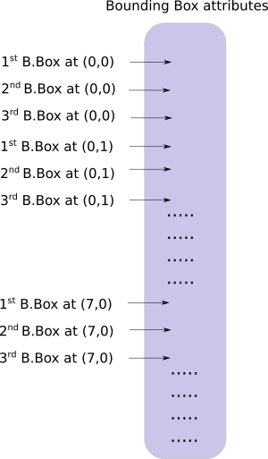
The output of YOLO is a convolutional feature map that contains the bounding box attributes along the depth of the feature map. The attributes bounding boxes predicted by a cell are stacked one by one along each other. So, if you have to access the second bounding of cell at (5,6), then you will have to index it by map[5,6, (5+C): 2*(5+C)]. This form is very inconvenient for output processing such as thresholding by a object confidence, adding grid offsets to centers, applying anchors etc.

Another problem is that since detections happen at three scales, the dimensions of the prediction maps will be different. Although the dimensions of the three feature maps are different, the output processing operations to be done on them are similar. It would be nice to have to do these operations on a single tensor, rather than three separate tensors.

To remedy these problems, we introduce the function predict_transform

Transforming the output

The function predict_transform lives in the file util.py and we will import the function when we use it in forward of Darknet class.

Add the imports to the top of util.py

from __future__ import division

import torch 
import torch.nn as nn
import torch.nn.functional as F 
from torch.autograd import Variable
import numpy as np
import cv2 

predict_transform takes in 5 parameters; prediction (our output), inp_dim (input image dimension), anchors, num_classes, and an optional CUDA flag

def predict_transform(prediction, inp_dim, anchors, num_classes, CUDA = True):

predict_transform function takes an detection feature map and turns it into a 2-D tensor, where each row of the tensor corresponds to attributes of a bounding box, in the following order.

Here’s the code to do the above transformation.

    batch_size = prediction.size(0)
    stride =  inp_dim // prediction.size(2)
    grid_size = inp_dim // stride
    bbox_attrs = 5 + num_classes
    num_anchors = len(anchors)

    prediction = prediction.view(batch_size, bbox_attrs*num_anchors, grid_size*grid_size)
    prediction = prediction.transpose(1,2).contiguous()
    prediction = prediction.view(batch_size, grid_size*grid_size*num_anchors, bbox_attrs)

The dimensions of the anchors are in accordance to the height and width attributes of the net block. These attributes describe the dimensions of the input image, which is larger (by a factor of stride) than the detection map. Therefore, we must divide the anchors by the stride of the detection feature map.

    anchors = [(a[0]/stride, a[1]/stride) for a in anchors]

Now, we need to transform our output according to the equations we discussed in Part 1.

Sigmoid the x,y coordinates and the objectness score.

    #Sigmoid the  centre_X, centre_Y. and object confidencce
    prediction[:,:,0] = torch.sigmoid(prediction[:,:,0])
    prediction[:,:,1] = torch.sigmoid(prediction[:,:,1])
    prediction[:,:,4] = torch.sigmoid(prediction[:,:,4])

Add the grid offsets to the center cordinates prediction.

    #Add the center offsets
    grid = np.arange(grid_size)
    a,b = np.meshgrid(grid, grid)

    x_offset = torch.FloatTensor(a).view(-1,1)
    y_offset = torch.FloatTensor(b).view(-1,1)

    if CUDA:
        x_offset = x_offset.cuda()
        y_offset = y_offset.cuda()

    x_y_offset = torch.cat((x_offset, y_offset), 1).repeat(1,num_anchors).view(-1,2).unsqueeze(0)

    prediction[:,:,:2] += x_y_offset

Apply the anchors to the dimensions of the bounding box.

    #log space transform height and the width
    anchors = torch.FloatTensor(anchors)

    if CUDA:
        anchors = anchors.cuda()

    anchors = anchors.repeat(grid_size*grid_size, 1).unsqueeze(0)
    prediction[:,:,2:4] = torch.exp(prediction[:,:,2:4])*anchors

Apply sigmoid activation to the the class scores

    prediction[:,:,5: 5 + num_classes] = torch.sigmoid((prediction[:,:, 5 : 5 + num_classes]))

The last thing we want to do here, is to resize the detections map to the size of the input image. The bounding box attributes here are sized according to the feature map (say, 13 x 13). If the input image was 416 x 416, we multiply the attributes by 32, or the stride variable.

prediction[:,:,:4] *= stride

That concludes the loop body.

Return the predictions at the end of the function.

    return prediction

#pytorch #deep-learning #data-science #developer #python