Linear Regression using TensorFlow 2.0

Are you looking for a deep learning library that’s one of the most popular and widely-used in this world? Do you want to use a GPU and highly-parallel computation for your machine learning model training? Then look no further than TensorFlow.

Created by the team at Google, TensorFlow is an open source library for numerical computation and machine learning. Undoubtedly, TensorFlow is one of the most popular deep learning libraries, and in recent weeks, Google released the full version of TensorFlow 2.0.

Python developers around the world should be about TensorFlow 2.0, as it’s more Pythonic compared to earlier versions. To help us get started working with TensorFlow 2.0, let’s work through an example with linear regression.

Getting Started

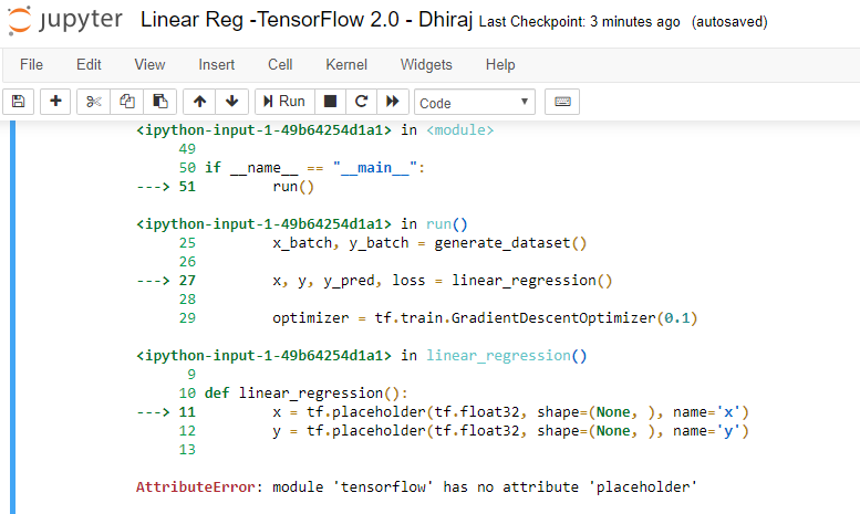
Before we start, let me remind you that if you have TensorFlow 2.0 installed on your machine, then the code written for linear regression using TensorFlow 1.x may not work. For example, tf.placeholder, which works with TensorFlow 1.x, won’twork with 2.0. You’ll get the error AttributeError: module ‘tensorflow’ has no attribute ‘placeholder’as shown in the image below_._

If you want to run the existing code (written in version 1.x) with version 2.0, you have two options:

1. Run your TensorFlow 2.0 installation in version 1.0 mode by using the below two lines of code:

import tensorflow.compat.v1 as tf
tf.disable_v2_behavior()

2. Modify your code to to work with version 2.0, as well as use the new and exciting features of version 2.0.

Linear Regression with TensorFlow 2.0

In this article, we’re going to use TensorFlow 2.0-compatible code to train a linear regression model.

Linear regression is an algorithm that finds a linear relationship between a dependent variable and one or more independent variables. The dependent variable is also called a label and independent variables are called features.

We’ll start by importing the necessary libraries. Let’s import three, namely numpy, tensorflow, and matplotlib, as shown below:

import numpy as np
import tensorflow as tf
import matplotlib.pyplot as plt

Before coding further, let’s make sure we’ve got the current version of TensorFlow ready to go.

Our next step is to create synthetic data for the model, as shown below. Assuming the equation of a line as y = mx + c , note that we’ve taken the slope of the line m as 2 and constant value c as 0.9. There is some error data we’ve introduced using np.random, as we don’t want the model to overfit as a straight line — this is because we want the model to work on unseen data.

# actual weight = 2 and actual bias = 0.9
x = np.linspace(0, 3, 120)
y = 2 * x + 0.9 + np.random.randn(*x.shape) * 0.3

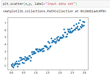
Let’s plot the data to see if it has linear pattern. We’re using Matplotlib for plotting. The data points below clearly show a pattern we’re looking for. Noticed that the data isn’t a perfectly straight line.

After visualizing our data, let’s create a class called Linear Model that has two methods: init and call. Init initializes the weight and bias randomly, and call returns the values, as per the straight line equation y = mx + c

class LinearModel:
    def __call__(self, x):
        return self.Weight * x + self.Bias
    
    def __init__(self):
        self.Weight = tf.Variable(11.0)
        self.Bias = tf.Variable(12.0)

Now let’s define the loss and train functions for the model. The train function takes four parameters: linear_model (model instance) , x (independent variable) , y (dependent variable), and lr (learning rate).

The loss function takes two parameters: y (actual value of dependent variable) and pred (predicted value of dependent variable).

Note that we’re using the tf.square function to get the square of the difference of y and the predicted value, and then we’re using the . tf.reduce_mean method to calculate the square root of the mean.

Note that the tf.GradientTape method is used for automatic differentiation, computing the gradient of a computation with respect to its input variables.
Hence, all operations executed inside the context of a tf.GradientTape are recorded.

def loss(y, pred):
    return tf.reduce_mean(tf.square(y - pred))

def train(linear_model, x, y, lr=0.12):
    with tf.GradientTape() as t:
        current_loss = loss(y, linear_model(x))

    lr_weight, lr_bias = t.gradient(current_loss, [linear_model.Weight, linear_model.Bias])
    linear_model.Weight.assign_sub(lr * lr_weight)
    linear_model.Bias.assign_sub(lr * lr_bias)

Here we’re defining the number of epochs as 80 and using a for loop to train the model. Note that we’re printing the epoch count and loss for each epoch using that same for loop. We’ve used 0.12 for learning rate, and we’re calculating the loss in each epoch by calling our loss function inside the for loop as shown below.

linear_model = LinearModel()
Weights, Biases = [], []
epochs = 80
for epoch_count in range(epochs):
    Weights.append(linear_model.Weight.numpy()) 
    Biases.append(linear_model.Bias.numpy())
    real_loss = loss(y, linear_model(x))
    train(linear_model, x, y, lr=0.12)
    print(f"Epoch count {epoch_count}: Loss value: {real_loss.numpy()}")

Below is the output during model training. This shows how our loss value is decreasing as the epoch count is increasing. Note that, initially, the loss was very high as we initialized the model with random values for weight and bias. Once the model starts learning, the loss starts decreasing.

And finally, we’d like to know the weight and bias values as well as RMSE for the model, which is shown below.

End notes

I hope you enjoyed creating and evaluating a linear regression model with TensorFlow 2.0.

You can find the complete code here.

Happy Machine Learning :)

#tensorflow #machine-learning #python