Introduction -

This article is in the continuation of my first article in which I have shown a complete procedure to perform Simple Linear Regression in detail. Now in this article, I am taking a little more complex data set (Advertising Data set) and going to show you How Multiple Linear Regression is prepared and using the information obtained from its diagnostic plot, how we proceed towards Orthogonal Polynomial Regression and obtain a better model for this data set.

This article consists of the following sections -

1. Loading Required Libraries
2. Loading Data set
3. Exploring Data set
4. Splitting Data set
5. Fitting Simple Linear Regression Model
6. Fitting Multiple Linear Regression Model with Diagnostic Plots and Statistical Tests
7. Fitting Orthogonal Polynomial Linear Regression Model with Diagnostic Plots and Statistical Tests
8. Making Predictions
9. Repeated 10-fold Cross Validation
10. Conclusion
11. Task for you (If interested)
12. Information about Next Article

I am going to use kaggle online platform for analysis work. You may use any software like R-studio or R-cran version.

1. Loading Required Libraries

It is not mandatory to load libraries in the beginning but I am doing it for simplicity.

# Loading required libraries
library(tidyverse)     # Pipe operator (%>%) and other commands
library(caret)         # Random split of data/cross validation
library(olsrr)         # Heteroscedasticity Testing (ols_test_score)
library(car)           # Muticolinearity detection (vif)
library(broom)         # Diagnostic Metric Table (augment)

2. Loading Data set

First of all, Load the data set in your online R-Session as follows -

Don’t know how to load data in kaggle online notebook, learn from here

# Loading Data set
data = read.csv("../input/advertising-dataset/advertising.csv" , header = T)

Advertising data set has been successfully loaded in the R-object “data”.

3. Exploring Data set

Make some understanding about the given data set as follows -

# Inspection of top 5-rows of data
head(data)

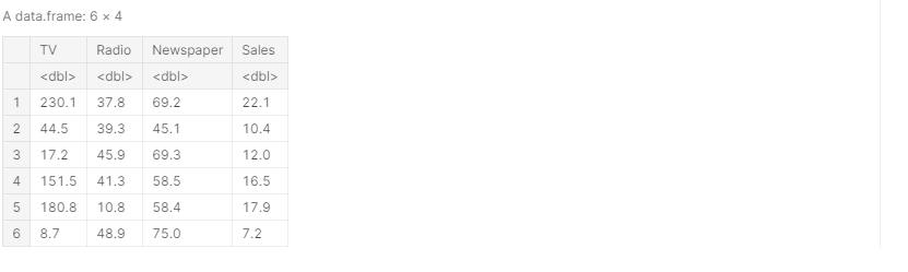
Output — 1

The above output shows top 5-rows of given data set. At this stage, just see the data and make some understanding as — There are four variables (TV,Radio,Newspaper,Sales) in the data set and all are numeric variables.

# Inspection of 5-bottom rows of data
tail(data)

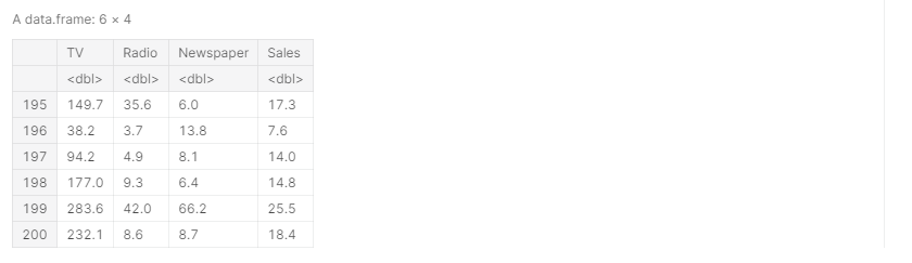
Output — 2

From the above output, it is clear that there are 200 rows in the data set and one more important point is that there are no rows that contains the information on something like “Totals”. It may be possible that in your data set there is a last row that contains the information of Totals of each column. Such rows are not useful in further analysis or during the model preparation. So, if there exists such row, just remove it from the data.

# Getting Structure of whole data set
str(data)

Output — 3

The above output gives information as-

1. There are 200 rows and 4 variables.
2. Variables are : TV,Radio,Newspaper,Sales
3. All are numeric variables.

# Checking Outliers
boxplot(data)

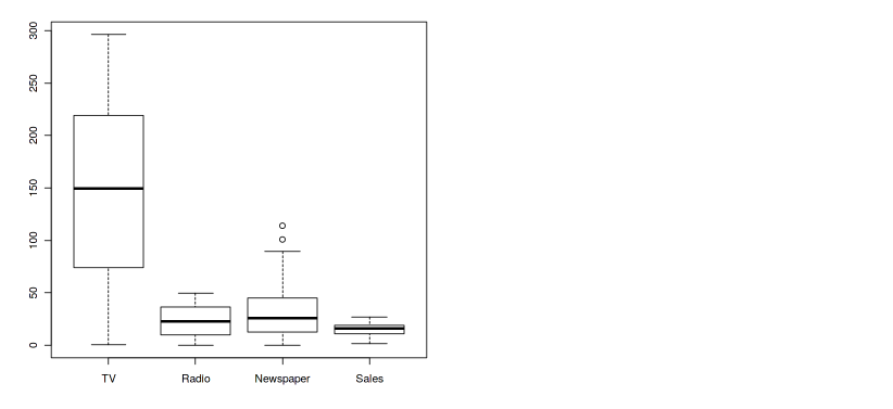
Output — 4

The above plot shows that two outliers are present in the variable “Newspaper”. Just remove these outliers by the following command -

# Removing Outliers
data <- data[-which(data$Newspaper %in%    boxplot.stats(data$Newspaper)$out), ]

Again, See the boxplot -

# Again Checking Outliers
boxplot(data)

Output — 5

Now, Outliers have been removed.

# Checking Missing Values
table(is.na(data))

Output — 6

The above output shows that there is no missing value in the given data set.

**Deciding the Target and Predictors **— It is always known to us which variable must be taken as Target and which as Predictors. This depends on the problem what you want to predict. I am taking here Sales as Target and rest variables as Predictors.

We have four numeric variables. Just take a look on scatter plot of these Variables as follows -

# Creating scatter plot matrix 
pairs(data , upper.panel = NULL)

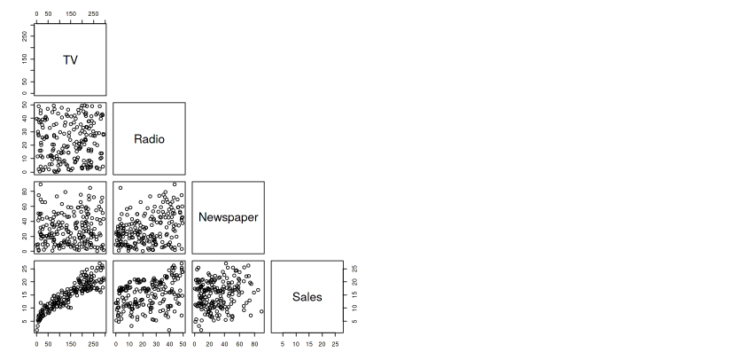
Output — 7

This output shows that -

1. No or very low linear relationship between TV and Radio variable.
2. Low linear relationship between TV and Newspaper variable.
3. Moderate linear relationship between Radio and Newspaper variable.
4. High linear relationship between TV and Sales , Radio and Sales , Newspaper and Sales.
5. A small curvilinear relationship is also present between TV and Sales as well as Radio and Sales.

Let’s get a more closer view to be more confident about existing relationship by plotting separate scatter plots -

# Scatter Plot between TV and Sales
plot(data$TV , data$Sales)

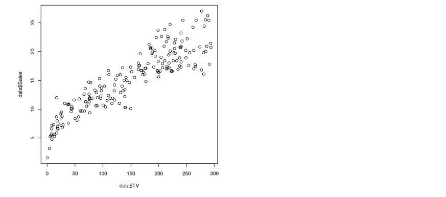
Output — 8

Notice, there is a small curvilinear relationship between TV and Sales.

# Scatter Plot between Radio and Sales
plot(data$Radio , data$Sales)

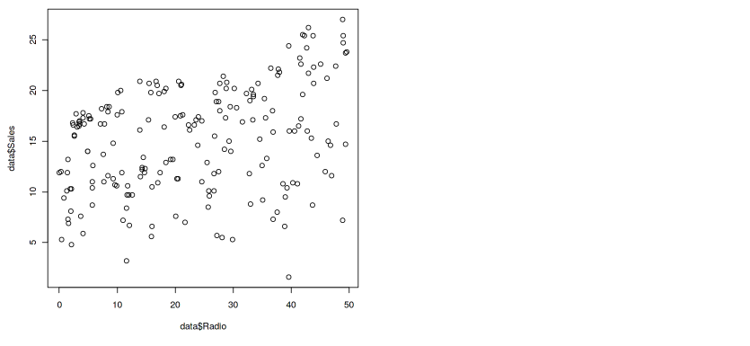
Output — 9

Notice, there is a curvilinear relationship between Radio and Sales.

# Scatter Plot between Newspaper and Sales
plot(data$Newspaper , data$Sales)

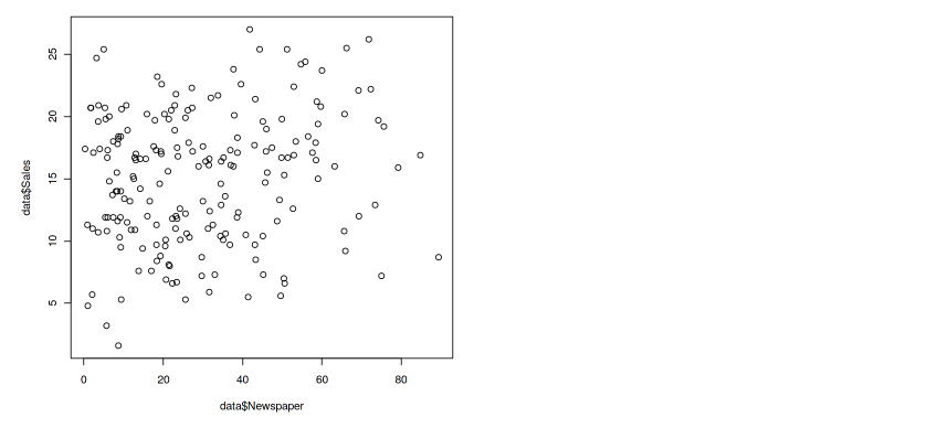
Output — 10

Low linear relationship between Newspaper and Sales variable.

# Scatter Plot between TV and Radio
plot(data$TV , data$Radio)

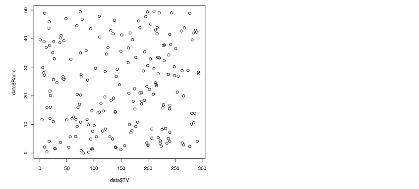
Output — 11

No linear relationship between TV and Radio variable.

#data-analysis #statistics #polynomial-regression #data-science #linear-regression #data analysis