Understanding the computational cost of kNN algorithm, with case study examples

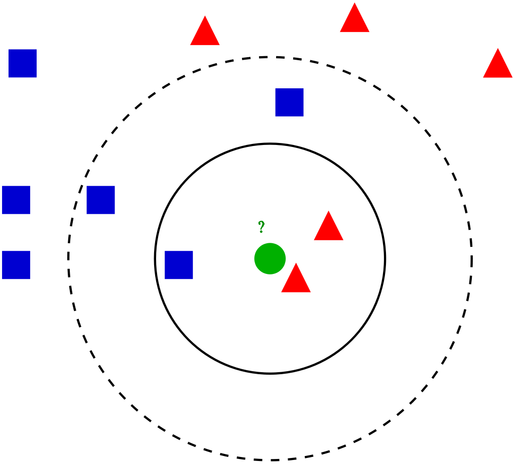
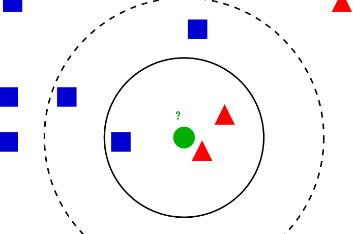
Visualization of the kNN algorithm (source)

Algorithm introduction

kNN (k nearest neighbors) is one of the simplest ML algorithms, often taught as one of the first algorithms during introductory courses. It’s relatively simple but quite powerful, although rarely time is spent on understanding its computational complexity and practical issues. It can be used both for classification and regression with the same complexity, so for simplicity, we’ll consider the kNN classifier.

kNN is an associative algorithm — during prediction it searches for the nearest neighbors and takes their majority vote as the class predicted for the sample. Training phase may or may not exist at all, as in general, we have 2 possibilities:

1. Brute force method — calculate distance from new point to every point in training data matrix X, sort distances and take k nearest, then do a majority vote. There is no need for separate training, so we only consider prediction complexity.
2. Using data structure — organize the training points from X into the auxiliary data structure for faster nearest neighbors lookup. This approach uses additional space and time (for creating data structure during training phase) for faster predictions.

We focus on the methods implemented in Scikit-learn, the most popular ML library for Python. It supports brute force, k-d tree and ball tree data structures. These are relatively simple, efficient and perfectly suited for the kNN algorithm. Construction of these trees stems from computational geometry, not from machine learning, and does not concern us that much, so I’ll cover it in less detail, more on the conceptual level. For more details on that, see links at the end of the article.

In all complexities below times of calculating the distance were omitted since they are in most cases negligible compared to the rest of the algorithm. Additionally, we mark:

• n: number of points in the training dataset
• d: data dimensionality
• k: number of neighbors that we consider for voting

Brute force method

Training time complexity: O(1)

**Training space complexity: **O(1)

Prediction time complexity: O(k * n)

Prediction space complexity: O(1)

Training phase technically does not exist, since all computation is done during prediction, so we have O(1) for both time and space.

Prediction phase is, as method name suggest, a simple exhaustive search, which in pseudocode is:

Loop through all points k times:
    1\. Compute the distance between currently classifier sample and 
       training points, remember the index of the element with the 
       smallest distance (ignore previously selected points)
    2\. Add the class at found index to the counter
Return the class with the most votes as a prediction

This is a nested loop structure, where the outer loop takes k steps and the inner loop takes n steps. 3rd point is O(1) and 4th is O(## of classes), so they are smaller. Therefore, we have O(n * k) time complexity.

As for space complexity, we need a small vector to count the votes for each class. It’s almost always very small and is fixed, so we can treat is as a O(1) space complexity.

#k-nearest-neighbours #knn-algorithm #knn #machine-learning #algorithms