Finite mixture models assume the existence of a latent, unobserved variable that impacts the distribution from which the data are generated. This idea has numerous practical applications: for instance, stock prices might change according to some assumed model, but the parameters of this model are likely to be different during bull and bear markets. In this case, the latent variable is the state of the economy, a somewhat undefined term, but a very impactful one.

Fitting finite mixtures to data comprises estimating the parameters of the distributions from which the data might come, as well as the probability of coming from each of them. This allows us to quantify and estimate important but undefined and unobservable variables, such as the already mentioned state of the economy! It is no easy task, though, with the standard maximum likelihood approach. Luckily, the clever expectation-maximization (or EM) algorithm comes to rescue.

This article is split into three parts, discussing the following topics:

1. What the EM algorithm is, how it works, and how to implement it in Python.
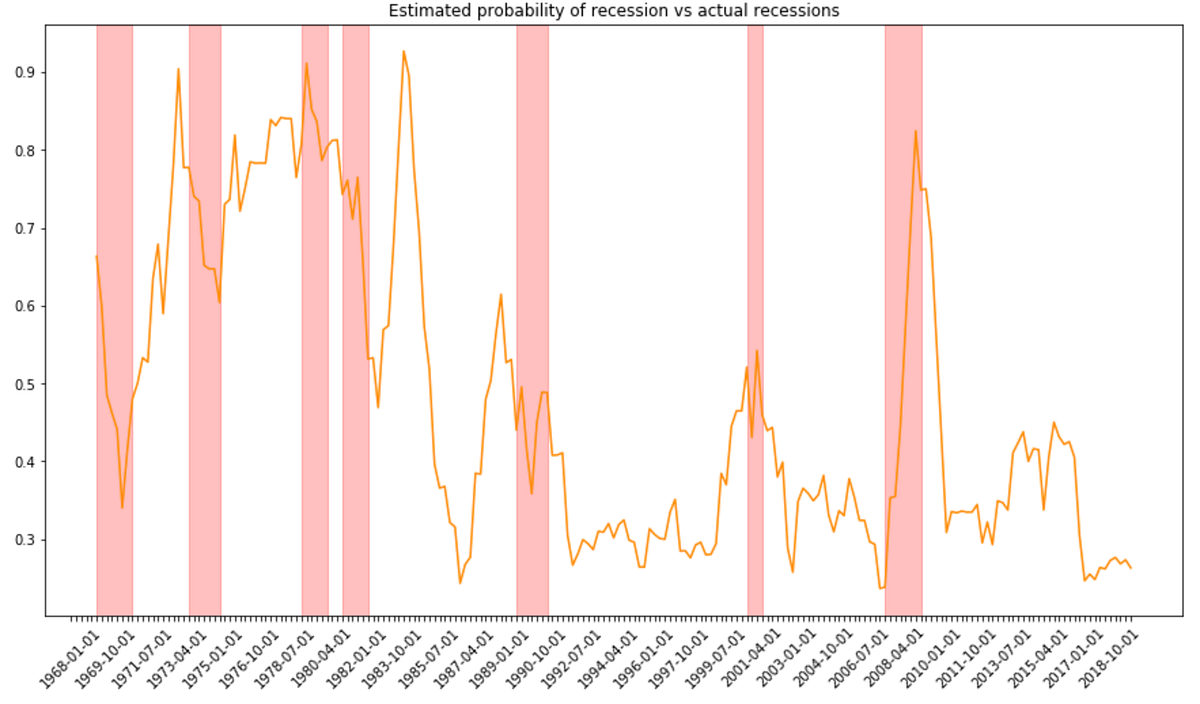
2. How to apply it in practice to estimate the state of the economy.
3. Appendix: the math behind the EM algorithm for curious readers.

Let’s dive straight in!

The Expectation-Maximization algorithm

We will discuss the EM algorithm using some randomly generated data first. Let’s start with the data generating process. Let’s say our data might come from two different normal distributions. One is described by a mean of -4 and a standard deviation of 2. For the other, the parameters are 11 and 3, respectively.

The data we actually observe are a mixture of the above two, defined as

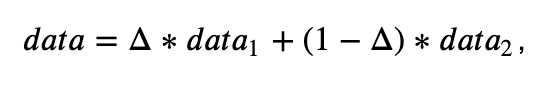
where Δ ∈ {0,1} with the probability 𝑝 of being 1. In our example, let’s set 𝑝 to 0.65. Consequently, if for a given data point Δ=1, it comes from the distribution 𝑑𝑎𝑡𝑎1, and if Δ=0, it comes from 𝑑𝑎𝑡𝑎2. Here, Δ is the latent variable we would not observe in reality which impacts the data generation process. Let’s generate some data according to this process and plot their histogram.

import numpy as np
	import pandas as pd
	from scipy.stats import norm
	import matplotlib.pyplot as plt
	import seaborn as sns

	data_1 = np.random.normal(-4, 2, 100),
	data_2 = np.random.normal(11, 3, 100)
	deltas = np.random.binomial(1, 0.65, 100)
	data = np.squeeze(deltas * data_1 + (1 - deltas) * data_2)

	sns.distplot(data, bins=15, kde=False, norm_hist=True)
	plt.show()
view raw
gaussian_mix_generated.py hosted with ❤ by GitHub

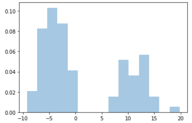
A quick look at the plot suggests the data might have arisen under a mixture of two normals. Hence, a finite mixture of two Gaussians seems to be the appropriate model for these data. Remember: all we observe is the data, and what we need to estimate are the parameters: 𝜇1, 𝜎1, 𝜇2, 𝜎2, and 𝑝, called the mixing probability, which is the probability of the data coming from one of the distributions — say the first one.

The likelihood of such data is very hard to maximize analytically. If you’d like to know why that’s the case, scroll down to the mathematical appendix. But there is another way — the EM algorithm. It’s a method providing the (possibly local) maximum of the log-likelihood function using an iterative two-step procedure:

• Expectation (E) step,
• Maximization (M) step.

In the E-step, we compute the so-called complete data likelihood function, based on the joint density of the data and the latent variable Δ. In the M-step, we maximize the expectation of this function. We repeat the two steps iteratively until the parameter estimates do not change anymore. All the mathematical derivations are relegated to the appendix below; for now, let me just offer you out-of-the-box formulas.

In the case of our mixture of two Gaussians, the E-step comprises computing the probability that 𝑝=1 given the other parameters, denoted as 𝑝𝑝1:

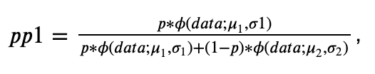
where 𝜙(𝑑𝑎𝑡𝑎;𝜇1,𝜎1) is the probability density of the data under the first distribution, a Gaussian with mean 𝜇1 and standard deviation 𝜎1. Let’s code it down:

# E-step: compute the conditional (posterior) probability that p = 1 (pp1), 
	# given the other parameters
	data_pdf_1 = norm.pdf(data, loc=mu_1, scale=sigma_1)
	data_pdf_2 = norm.pdf(data, loc=mu_2, scale=sigma_2)
	pp1 = (p * data_pdf_1) / (p * data_pdf_1 + (1 - p) * data_pdf_2)
view raw
EM_E_step.py hosted with ❤ by GitHub

The maximizing formulas applied in the M-step are as follows (scroll to the bottom for the derivations):

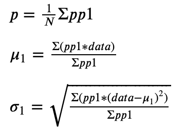
The formulas for 𝜇2 and 𝜎2 are the same, except that they use (1−𝑝𝑝1) in place of 𝑝𝑝1. Let’s translate it into Python:

# M-step: maximize the pp1 with respect to the parameters
	p = np.mean(pp1)
	mu_1 = np.sum(pp1 * data) / np.sum(pp1)
	mu_2 = np.sum((1 - pp1) * data) / np.sum((1 - pp1))
	sigma_1 = np.sqrt(np.sum(pp1 * (data - mu_1)**2) / np.sum(pp1))
	sigma_2 = np.sqrt(np.sum((1 - pp1) * (data - mu_2)**2) / np.sum((1 - pp1)))
view raw
EM_M_step.py hosted with ❤ by GitHub

As you see, the E-step conditions on the parameters 𝜇1, 𝜎1, 𝜇2, 𝜎2, and 𝑝 and the M-step updates them. To get it started, we need to initialize these parameters before we run the first E-step iteration. A popular choice is to set the means 𝜇 to any random data points drawn from the data, the standard deviations 𝜎 to the standard deviation of the data, and 𝑝 to 0.5:

# Initial guesses for the parameters
	mu_1 = np.random.choice(data)
	mu_2 = np.random.choice(data)
	sigma_1 = np.std(data)
	sigma_2 = np.std(data)
	p = 0.5
view raw
EM_init_params.py hosted with ❤ by GitHub

We have now coded the entire EM algorithm! Let’s put all this code together into a class called TwoGaussiansMixture() with a fit() method which takes data and num_iter as arguments, initializes the parameters and iterates through the E and M steps for num_iter iterations. The class will also have three other utility methods:

• predict(), which takes some data x and produces the predicted PDF of our fitted Gaussian mixture for these data,
• get_mixing_probability(), which takes some data x and returns the probability of coming from one of the distributions for each data point,
• plot_predictions_on_data(), which plots the PDF produced by predict() on top of the histogram of the original data.

#data-science #statistics #time-series-analysis #algorithms