In the following project, I applied three different machine learning algorithms to predict the quality of a wine. The dataset I used for the project is called _Wine Quality Data Set _(specifically the “winequality-red.csv” file), taken from the UCI Machine Learning Repository.

The dataset contains 1,599 observations and 12 attributes related to the red variants of the Portuguese “Vinho Verde” wine. Each row describes the physicochemical properties of one bottle of wine. The first 11 independent variables display numeric information about these characteristics, and the last dependent variable revels the quality of the wine on a scale from 0 (bad quality wine) to 10 (good quality wine) based on sensory data.

Since the outcome variable is ordinal, I chose logistic regression, decision trees, and random forest classification algorithms to answer the following questions:

1. Which machine learning algorithm will enable the most accurate prediction of wine quality from its physicochemical properties?
2. What physicochemical properties of red wine have the highest impact on its quality?

---

For the following project, I used the R programming language to explore, prepare, and model the data.

Importing the dataset

Once the working directory is set and the dataset is download into our computer, I imported the data.

#Importing the dataset
data <- read.csv('winequality-red.csv', sep = ';')
str(data)

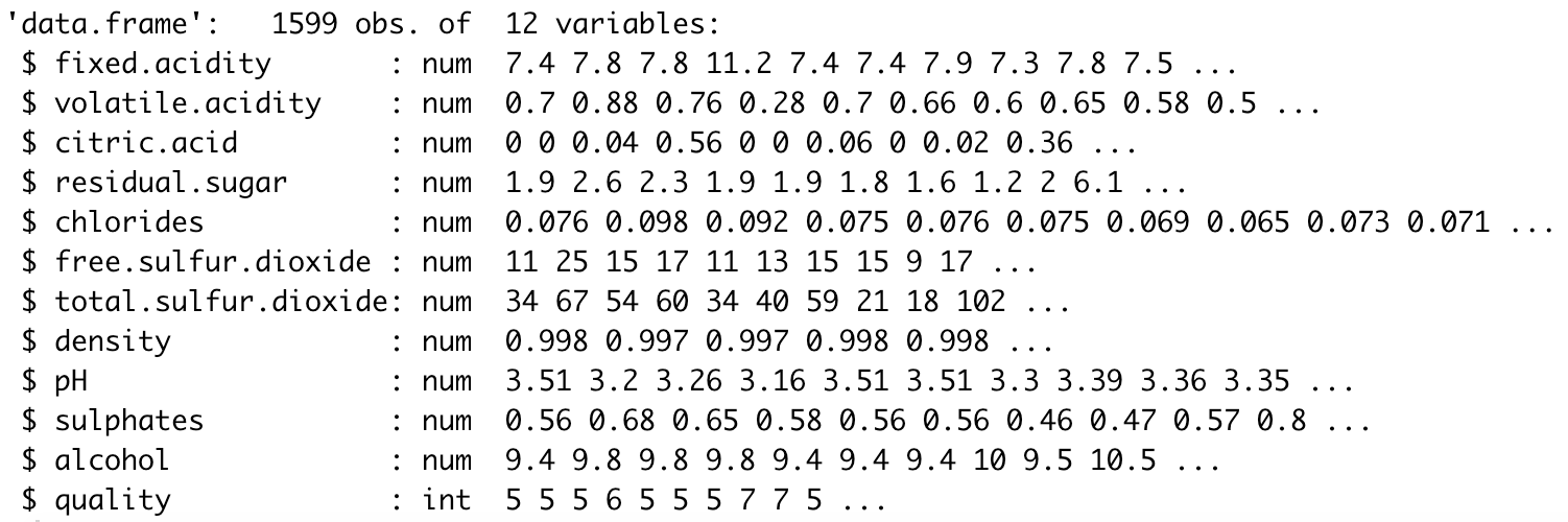
Results from the srt() function

With the str() function, we could see that all the variable types are numerical, which is the correct format except the outcome variable. I proceed to transform the dependent variable into a binary categorical response.

#Format outcome variable
data$quality <- ifelse(data$quality >= 7, 1, 0)
data$quality <- factor(data$quality, levels = c(0, 1))

The arbitrary criteria I selected to modify the levels of the outcome variable is as follows:

1. Values above or equal to seven will be changed to 1, meaning a good quality wine.
2. On the other hand, amounts less than seven will be converted to 0 and will indicate bad or mediocre quality.

Furthermore, I modified the type of the variable “quality” to factor, indicating that the variable is categorical.

Exploratory data analysis (EDA)

Now, I proceed to develop an EDA on the data to find essential insights and to determine specific relationships between the variables.

First, I developed a descriptive analysis where I collected the five-number summary statistics of the data by using the summary() function.

#Descriptive statistics
summary(data)

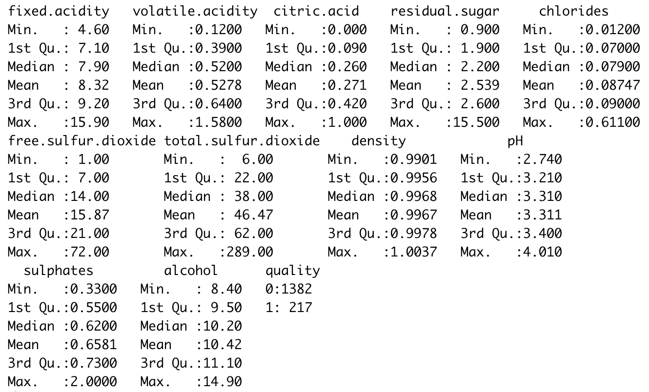
Five-number summary values of each of the variables in the data

The image shows the five-number summary values of each of the variables in the data. In other words, with the function, I obtained the minimum and maximum, the 1st and 3rd quartile, the mean, and the median values of the numerical variables. Additionally, the summary shows the frequency of the level of the dependent variable.

Next, I developed a univariate analysis, which consists of examining each of the variables separately. First, I analyzed the dependent variable.

To analyze the outcome variable, I developed a bar plot to visualize the frequency count of the categorical levels. Also, I generated a table of frequency count to know the exact amount and percentage of value that are in the different levels in each category.

#Univariate analysis
  #Dependent variable
    #Frequency plot
par(mfrow=c(1,1))
barplot(table(data[[12]]), 
        main = sprintf('Frequency plot of the variable: %s', 
                       colnames(data[12])),
        xlab = colnames(data[12]),
        ylab = 'Frequency')
#Check class BIAS
table(data$quality)
round(prop.table((table(data$quality))),2)

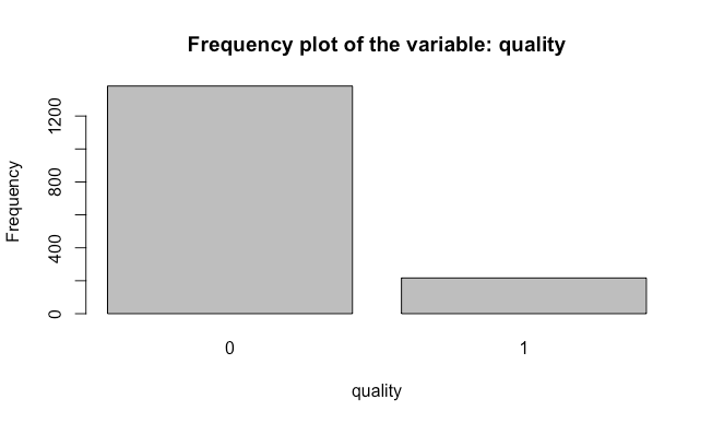
Frequency plot to analyze the dependent variable

Analyzing the plot, I stated that the dataset has a considerably higher amount of 0 values, indicating that the data has more rows that represent a bad quality of the wine. In other words, the data is biased.

Further, by analyzing the tables, I declared that the data has 1,382 rows that were qualified as a bad quality wine and 217 as a good quality wine. Likewise, the dataset contains approximately 86% of 0 outcome values and 14% of 1 outcome values.

In that sense, it is necessary to take into consideration that the dataset is biased. That is why it is essential to follow a stratified sampling method when splitting the data into the train and test set.

Now, I proceed to analyze the independent variables. To develop the analysis, I chose to create boxplots and histogram plots for each variable. These visualizations will help us identify the location of the five-number summary values, the outliers it possesses, and the distribution that the variable follows.

#machine-learning #r #supervised-learning #data-science #towards-data-science #deep learning