This article is part 3 in my series detailing the use and development of SAEMI, a web application I created to perform high throughput quantitative analysis of electron microscopy images. You can check out the app here and its github here. Also, check out part 1 here (where I talk about the motivation behind creating this app) and part 2 here (where I give a walk-through of how to use the app). In this article, I will talk about how I trained a deep learning model to segment electron microscopy (EM) images for quantitative analysis of nanoparticles.

Choosing a Dataset

In order to train my model, I used a data-set taken from NFFA-EUROPE with over 20,000 Scanning Electron Microscopy (SEM) images taken from CNR-IOM in Trieste, Italy. This was one of the only large databases of EM images that I could actually access for free as you can imagine, most EM images are subject to strong copyright issues. The database consists of over 20,000 SEM images separated into 10 different categories (Biological, Fibres, Films_coated_Surface, MEMS_devices_and_electrodes, Nanowires, Particles, Patterned_surface, Porous_Sponge, Powder, Tips). For my training, however, I limited the training images to only be taken from the Particles category, which consisted of just under 4000 images.

One of the main reasons for this is because for almost all of the other categories, there wasn’t actually a way to obtain a useful size distribution from the image. For example, consider the EM image of fibres shown in Figure 1a. After segmenting the image, I could calculate the sizes of each fibre within the image, but you can also clearly see that the fibres extend out past the image. Therefore, the sizes I calculate are limited to what’s presented in the EM image and I can’t extract how long the fibres are from the image alone.

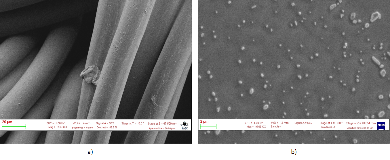
Compare that to Figure 1b of the EM image of particles where the sizes shown in the image are clearly the size of the entire particle. Not only that, but images in this category tended to have the least degree of occlusion which made labeling and training much easier.

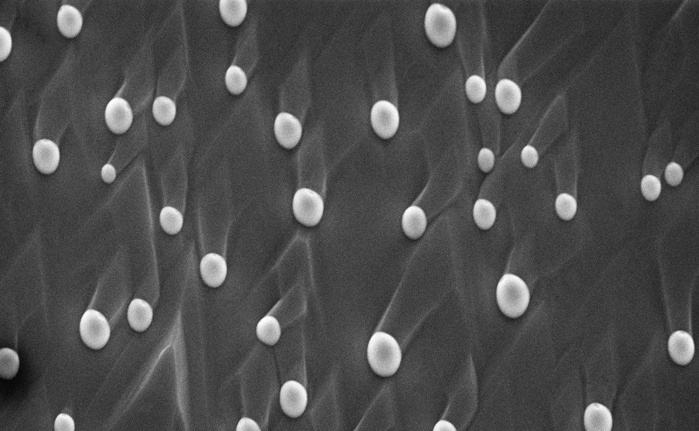
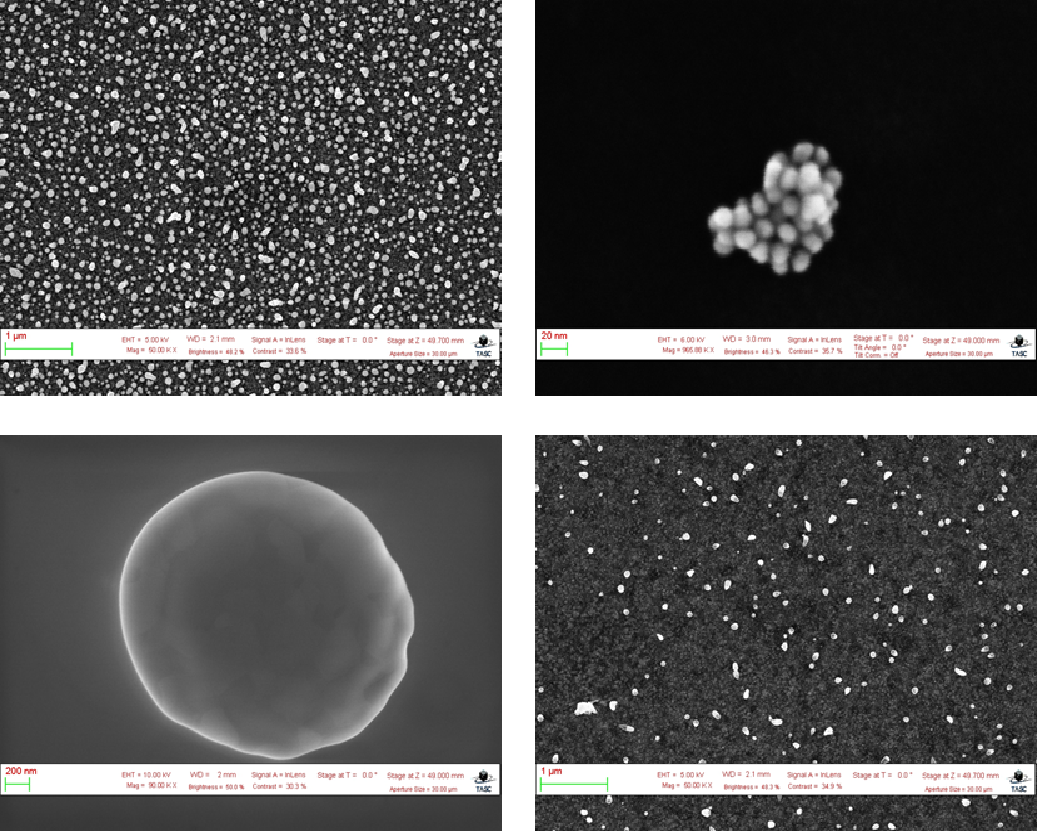
Within the Particles category, all the images were 768 pixels tall and 1024 pixels wide. Most of the particles were roughly circular in shape, with some images featuring hundreds of particles and other images featuring only one particle. The size of the particles in pixels were also quite varied due to differences in the magnification which ranged from 1 micron to 10 nanometers. An example of some of the particle images in the data-set is shown in Figure 2 below:

Removing the Banners

To begin the training process, the raw images first had to be preprocessed. For the most part, this meant removing the banners that contained image metadata while retaining as much useful image data as possible. To accomplish this, I used a technique called “reflection padding”. Essentially, I replaced the banner region with its reflections along the top and bottom. An example of this is shown in Figure 3 with the reflections highlighted in red.

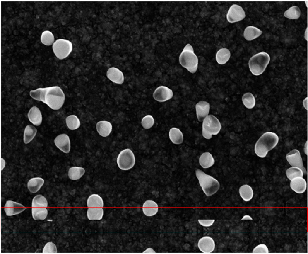
Fig 3 Example of reflection padding. source: CNR-IOM (CC-BY)

In order to perform this transformation, however, I first had to detect the banner regions using OpenCV. To start, I took my image and created a binary mask of the image where all pixel values above 250 becomes 255 and all pixels below the threshold becomes 0. The code used to perform this is shown below along with the result in Figure 4.

import cv2

# convert image to grayscale
grayscale = cv2.cvtColor(img, cv2.COLOR_BGR2GRAY)
# create binary mask based on threshold of 250
ret, binary = cv2.threshold(gray, 250, 255, cv2.THRESH_BINARY)

While thresholding was already fairly effective in finding the banner region, I could still detect some elements of the image that weren’t part of the banner. To make sure only the banner region was detected and nothing else remained, I used erosion and dilation on the thresholded image to find where the vertical and horizontal lines are within the image. Erosion is an image processing technique where a kernel of a given size is scanned across an image. As the kernel travels along the image, the minimum pixel value is found and the pixel value at the center is replaced by that minimum. Dilation is a similar operation but the maximum pixel value is used instead.

The code to detect vertical and horizontal lines are shown below along with their results in Figure 5.

#machine-learning #data-science #data analysis