How do neural networks classify images so well? Despite much progress on the accuracy, we haven’t been able to explain the inner workings of neural networks yet.

A convolutional neural network (ConvNet) is just a composition of simple mathematical functions — building blocks (BB). Those BBs by themselves are much easier to understand and we can get an idea of what they are doing by carefully looking at their parameters (weights) and by observing how they transform their inputs.

Since each BB is (mostly) explainable by itself, and a ConvNet is just a composition of those BBs, we should be able to compose all small explanations of the BBs and build an understanding of the entire mechanism of how ConvNet works, right?

This is the question that I wanted to explore. As a simple example, I wanted to understand how a ConvNet trained on MNIST classifies images of digits and inspired by the trained ConvNet, to build a ConvNet by hand (without training) based on much simpler BBs which would imitate the BBs of the original ConvNet but they would be more constrained and thus hopefully more explainable.

I started by _dissecting a ConvNet _trained on MNIST (which I will call SimpleConvNet) where I found that one of the convolutional layers can be omitted altogether because it just replicates the outputs of the previous convolutional layer. I also found the duality of the BBs, i.e. BBs are used both to detect patterns and detect the location of those patterns. After understanding the BBs of SimpleConvNet, I started building a ConvNet by hand (which I will call HandNet) consisting of more constrained (thus easier to tweak than using backprop) BBs. I found that the handmade ConvNet performs much worse but after fine-tuning, its accuracy becomes on par with SimpleConvNet. The advantage of HandNet over SimpleConvNet is that it’s much easier to understand and explain its inner workings.

In this article, I will explain the dissection of SimpleConvNet in detail. In Part 2, I will show how I built the HandNet using more constrained BBs.

There is a Colab notebook for this article if you want to follow along with the code, tweak the code, or perform a similar dissection of your network.

Here is the outline of the rest of the article

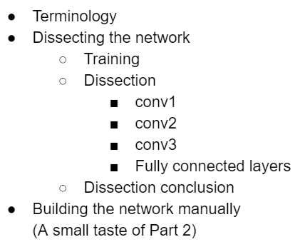
Terminology

First, some terminology that I will use in the rest of the article:

I use PyTorch notation for convolutional layers: Input is of shape (N, _C_in​, H, W). The output is of shape (N, _C_out​, _H_out​, _W_out​). The convolution will be said to have Cin **_inner _**channels and Cout outer channels.

I will use 1-based indexing throughout this article because it makes the diagrams easier to follow.

Dissecting the network

Training

I started by training a ConvNet with a fairly simple architecture shown below.

(conv1 + relu + maxpool) → (conv2 + relu + maxpool) → (conv3 + relu + maxpool) → flattening → fc4 → fc5 → log_softmax. Image generated using this tool.

I was mainly interested in dissecting the convolutional layers because the fully connected layers are pretty straightforward since they just implement the linear combination. Looking at convolutions, we see that conv2 weights (with shape [64, 32, 5, 5]) for example, will consist of 64x32=2048 grids of size 5x5. This is a fairly large number of grids to label manually, so I decided to reduce the size of the network.

I iteratively pruned outer channels (see **Terminology **section for the explanation of outer channels) of conv. layers based on the criteria described below:

• The ones that have small activation variation.
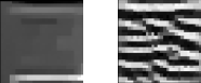
• The ones that look like noise (as opposed to the ones that look like pattern detectors like Gabor filters).

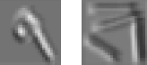
Examples of grids from conv1 that look like noise (left) vs a pattern detector (right)

• The outer channels that have “plain” superstimuli (superstimuli are described in the Feature Visualization section of the Curve Detectors).

Examples of plain superstimulus (left) vs superstimulus that has a clear pattern (right)

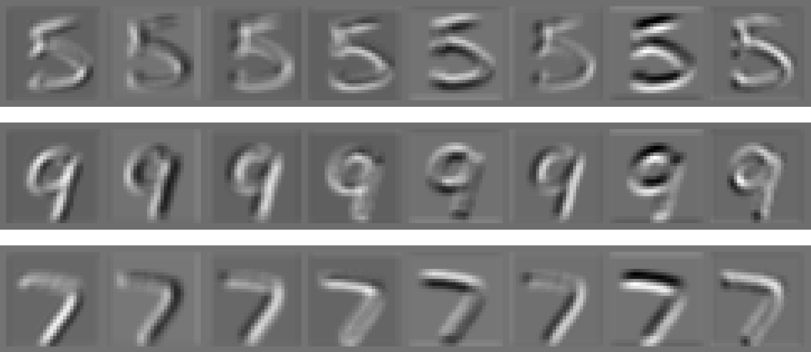
• The outer channels that don’t selectively respond to inputs from MNIST or curated synthetic inputs.

Examples of selective response. Left: MNIST digit — the conv. responds selectively to the diagonal part of digit 9. Right: Curated synthetic input — the conv. responds selectively to the vertical line.

*** I pruned the entire outer channel and not just some inner channels because removing only some inner channels within a given outer channel makes the convolution operation irregular and kind of ugly 😬.

After each iteration of pruning, the accuracy of the ConvNet dropped slightly, but retraining the network quickly brought back the accuracy before the pruning, suggesting many weights are useless. The pruning removes useless weights which is essentially noise and it brings the essence of classification closer to the surface. The hope is that there should be just a small number of pathways that are used for classification, the rest is noise.

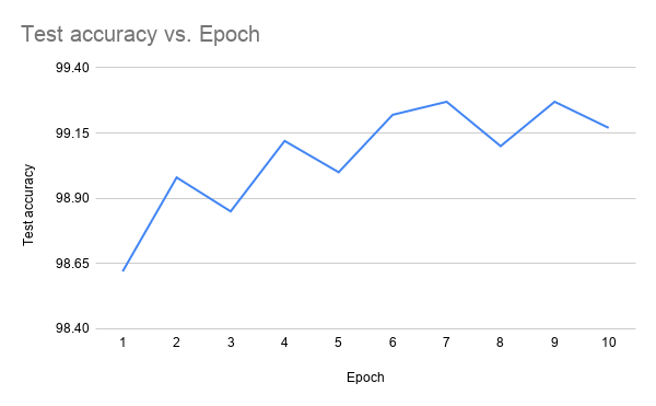
Retraining the ConvNet after each iteration of pruning brings back the pre-pruning accuracy

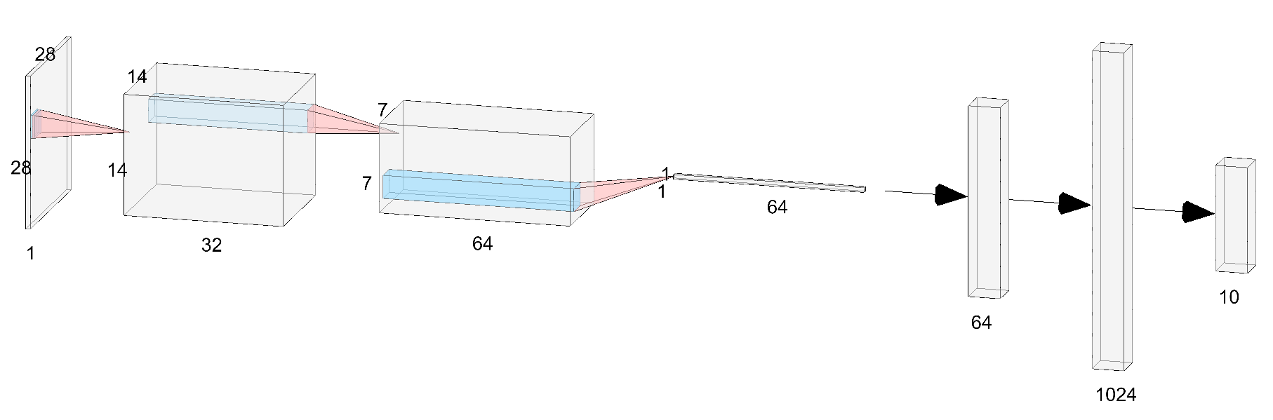
Final architecture (after 7 iterations of pruning) is shown below. As you can see, the depth of each layer has been significantly decreased.

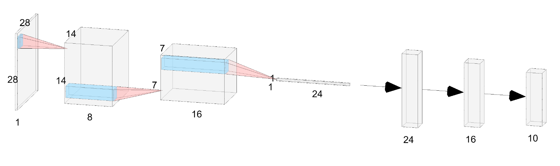
Final architecture after pruning. Image generated using this tool.

We have 3 conv layers, followed by flattening, followed by 2 fully connected (fc) layers. (conv1 + relu + maxpool) → (conv2 + relu + maxpool) → (conv3 + relu + maxpool) → flattening → fc4 → fc5 → log_softmax

---

Dissection

Conv1

Let’s start by looking at the weights of conv1 which has shape [8, 1, 5, 5] (8 outer channels, 1 inner channel, 5x5 grids):

and their activations on random input from MNIST:

and their activations on synthetic input (in the image, I used a line for each direction: horizontal, vertical, and 2 diagonals):

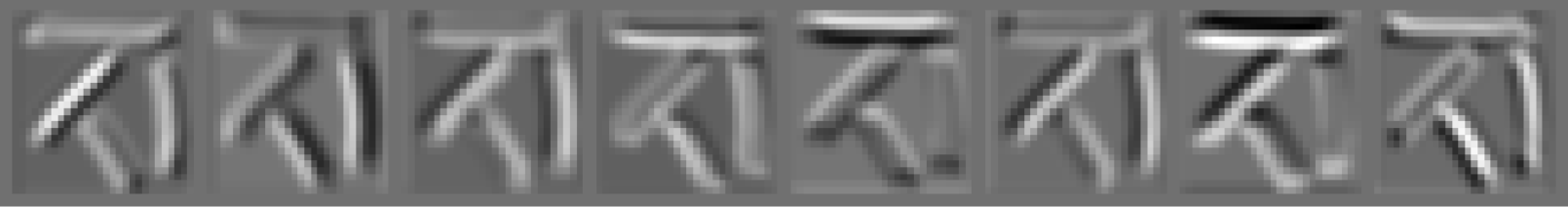
The 3 images above strongly suggest that the first filter in conv1 detects lines at slope=45° (you can see that just from the weights — the pattern resembles a line at slope=45°). The coordinate frame used for the angles is shown below:

Similarly, the second and third filters are detecting vertical lines. However, the difference between them is that the second filter detects the left side of the vertical line, and the third filter detects the right side. If we do this exercise for all filters, we can get the following mapping from the index (1-based) of the filter to the pattern that it’s detecting:

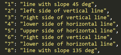
Explanations of conv1 filters — mapping from index of filter to pattern that it’s detecting

We can see that some patterns are repeating: Filters with index=3 and 6 are detecting the same “right side of vertical line” and filters with index= 4 and 7 are detecting the same “lower side of horizontal line”. Notice also that these filters as a collection seem to span the entire space of line directions albeit a very discrete one (with increments of 45 degrees). (the space consisting of the following angles: [0, 45, 90, 135])

Keep in mind that conv2 will not see the output of conv1 directly. There are ReLU and MaxPool between them. So the negative values and most of the low positive values will disappear from the output of conv1 when conv2 sees it.

---

Conv2

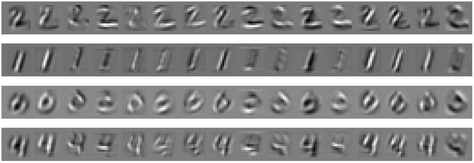
Conv2 shape is [16, 8, 5, 5] (16 outer channels, 8 inner channels, 5x5 grids). Now, we can’t just look at the weights of conv2 because that would require visualizing 16*8=128 filters of size 5x5 which is a little too much. Besides, a conv2 outer channel (see Terminology section for the definition of the outer channel) is not as simple as just a convolution of a filter with an image (which was the case for conv1), instead, it’s a linear combination of such convolutions (because unlike conv1, conv2 inner channels is not equal to one) which makes it harder to visualize conv2’s mechanism by just looking at the 128 filters. So, for now, we will skip visualizing the weights directly. Instead, let’s start with visualizing the superstimuli (see Feature Visualization for the definition of superstimuli) for each of conv2’s outer channels (there are 16 of them).

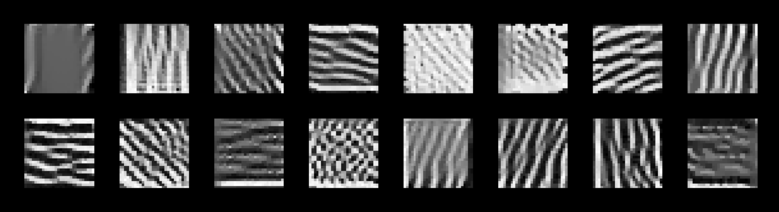
Superstimuli for conv2 outer channels

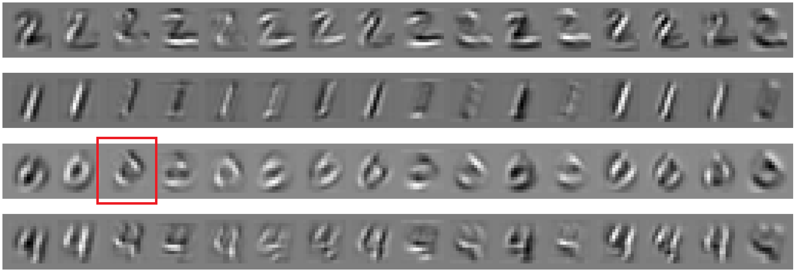
The superstimuli can give a hint of what each outer channel of conv2 is trying to detect. For example, it suggests that the outer channel with index=3, we’ll call it conv2_3, is detecting diagonal patterns at slope=135°.

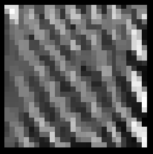
Superstimulus of conv2_3

The activations of conv2 outer channels on random input from MNIST:

Let’s look at activations of conv2_3. We already saw from its superstimuli that it’s trying to detect diagonal patterns at slope=135°. The activations above seem to confirm this hypothesis — only the diagonal part of digit 0 at slope=135° is highlighted by this outer channel:

Let’s look more closely at how conv2_3 implements this:

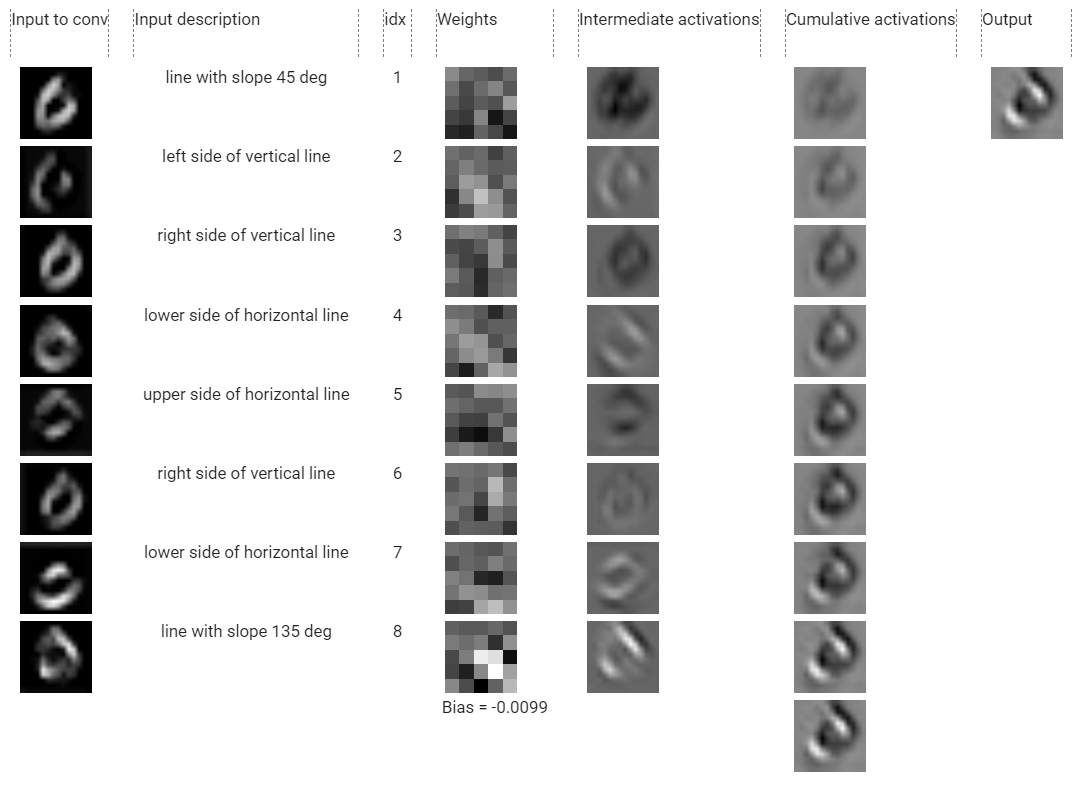
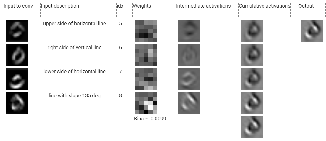
Dissected activation of conv2_3

Let me explain this beast of a diagram.

• First column: the total input to conv2 ( i.e. maxpool(relu(output of conv1)) ). We will denote row j in this column by x_j.
• Second column: the description of each outer channel of conv1 which we discovered in the previous section. This column is supposed to describe the first column (even though it’s not perfect).
• Third column: the index (1-based) of the inner channel of conv2_3.
• Fourth column: the weights of each of the inner channel of conv2_2. We will denote row j in this column by w_j.
• Fifth column: Row j in this column is the convolution of x_j with w_j, that is a_j=x_j ∗ w_j. (a for activation)
• Sixth column: Row j in this column is the accumulation of all a_j’s. That isc_j=Σ a_k from k=1 to k=j (c for cumulative). And the last row is _c_8= Bias + Σ a_k from k=1 to k=8 _(bias is from the last row of the fourth column).
• The seventh column is the output of conv2_3. It’s just the last row of the sixth column duplicated. We will denote it y. Essentially, conv2_3 just sums up the individual convolutions of its inner channels (x_j ∗ w_j)

*** The color scale is re-normalized within each column for easier comparison. (So the first rows of fifth and sixth columns actually have the same values but they look different because of different color normalizations applied to them).

Let’s start analyzing each row.

• a_1=x_1∗ w_1 does not convey any meaning and by looking at the total output ofconv2_3, which is y,it does not look like a_1 has any effect on y.This is most likely due to_ a_1_ being overwhelmed by other a__j_’s. So let’s ignore this row.
• w_2 seems to detect lines with slope=135_°. By looking at a_2 we see that it’s true but a_2 is very weak thus we don’t see much contribution from a_2 to the total output y_. We will also ignore this row.
• By looking at a_3 it seems that row with index=3 just negates its input x_3 which is “right side of vertical line”. It implements this negation by having a strongly negative vertical line close to the center of its grid of weights (column 4, row 3). So we will denote a_3’s description as neg(“right side of vertical line”).
• _a_4 _is the first significant contribution to y. You can see that starting from _c_4 and everything below it has those 2 bright blobs that are present in y (the parts of digit 0 at slope=135°). w_4 just looks for lines at slope 135° and this overlaps with its input x_4, _thusline with slope 135° is highlighted in _a_4. _So we just see more of “line with slope 135 deg” in a_4.

*** (x_4’s description is_ “lower side of horizontal line” but in this particular image conv1_4 seems to detect diagonal lines — you can never be 100% certain with neural networks ¯_(ツ)/¯. Actually, if you carefully look at the weight of conv1_4 (shown below), it has a very vague hint that it’s detecting lines with slope 135° (highlighted in the figure below). I call these types of patterns secondary functions of conv. filters. I will mostly omit these by concentrating only on the primary ones because they are usually stronger than the secondary ones. But we always have to keep in mind that there might be secondary, or even more patterns that a conv. filter detects).

Secondary function of conv1_4

We are halfway through conv2_3. I will replicate the diagram of conv2_3 dissection so that you scroll a little less:))

Dissected activation of conv2_3

• 5th row: _w_5 _negates _x_5 _by having a strongly negative horizontal line in the _w_5 _grid which (negatively) matches _x_5 _(which is “upper side of horizontal line”). We’ll call a_5’s description neg(“upper side of horizontal line”).
• _w_6 _looks like it detects vertical lines but it’s ambiguous. _a_6 _does not look very strong either, thus it does not contribute to _y _significantly so we will ignore this row as well.
• _w_7 _has a horizontal bright line so it’s most likely detecting horizontal lines which again matches with its input _x_7 _(“lower side of horizontal line”). The net contribution _a_7 _is the replicated _x_7 _but this contribution is weak compared to other a_j’swhich you can see from it’s faded color in the 5th column. Thus we will label this row as weak(“lower side of horizontal line”).
• The final row is by far the most significant contribution which you can see from the dissected activations column. It has the strongest influence on the net output y. The magnitude of _a_8 _is much bigger than other a_j’s because w_8’s magnitude (and contrast) is much bigger than other w_j’s. You can see from the grid of _w_8 (shown below as well) that it has a very high contrast between the negative values and positive values (very bright and very dark blobs around) thus it has a very strong tendency to detect lines with slope 135_°. What’s more, is that the pattern that _w_8 _is trying to detect matches its input (again!) _x_8 _which is “line with slope 135 deg”. This just reinforces the pattern detected by _x_8 and we see a very strong selectivity to lines with slope 135_° in a_8.

#deep-learning #image-recognition #visualization #mnist #convnets #visual studio code