Plot legends are essential for properly annotating your figures. Luckily, MATLAB/Octave include the legend() function which provides some flexible and easy-to-use options for generating legends. In this article, I cover the basic use of the legend() function, as well as some special cases that I tend to use regularly.

The source code for the included examples can be found in the GitHub repository.

Basic Use of Plot Legends

The _legend() _function in MATLAB/Octave allows you to add descriptive labels to your plots. The simplest way to use the function is to pass in a character string for each line on the plot. The basic syntax is: legend( ‘Description 1’, ‘Description 2’, … ).

For the examples in this section, we will generate a sample figure using the following code.

x = 0 : 0.1 : ( 2pi ); 
plot( x, sin( x ), 'rx', 'linewidth', 2 ); 
hold on; 
plot( x, cos( x/3 ) - 0.25, 'bs', 'linewidth', 2 ); 
plot( x, cos( 4x )/3, '^g', 'linewidth', 2 );
hold off;
xlim( [ 0, 2*pi ] );
grid on;
title( 'Sample Plot' );
set( gca, 'fontsize', 16 );

A legend can be added with the following command.

legend( 'Line 1', 'Line 2', 'Line 3' );

In addition to specifying the labels as individual character strings, it is often convenient to collect the strings in a cell array. This is most useful when you are programmatically creating the legend string.

legStr = { 'Line 1', 'Line 2', 'Line 3' };
legend( legStr );

For convenience, this method will be used for the rest of the examples. The resulting figure looks like this.

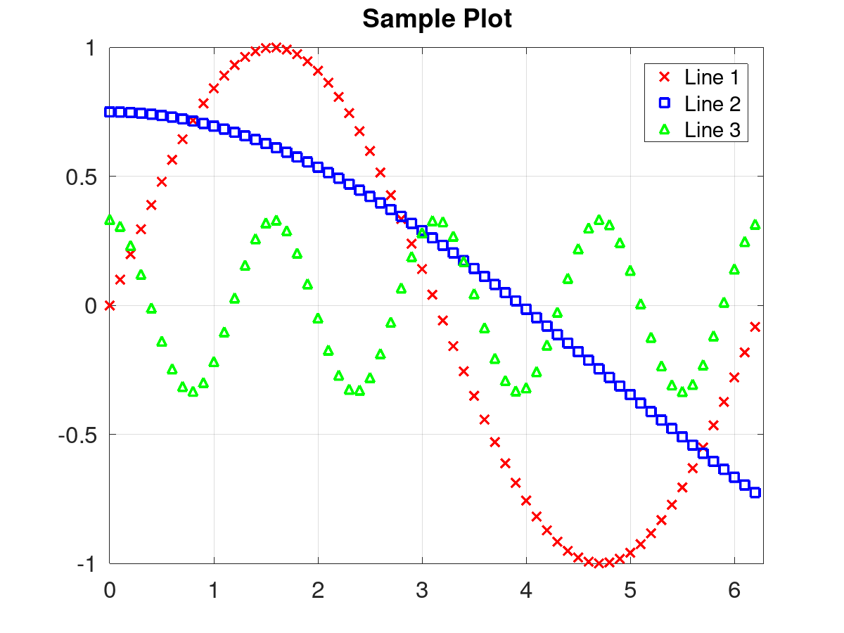
Image by author

By default the legend has been placed in the upper, right corner; however, the ‘location’ keyword can be used to adjust where it is displayed. The location is selected using a convention based on the cardinal directions. The following keywords can be used: north, south, east, west, northeast, northwest, southeast, southwest. The following code snippet would place the legend in the center top of the plot.

legend( legStr, 'location', 'north' );

Similarly, all of the other keywords can be used to place the legend around the plot. The following animation illustrates all of the different keywords.

Image by author

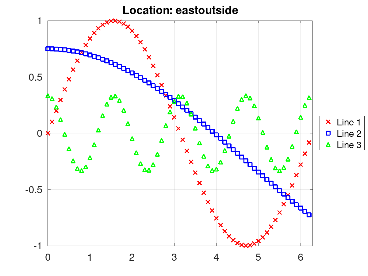
The keyword ‘outside’ can also be appended to all of the locations to place the legend outside of the plot. The next image shows an example with the legend on the east outside.

legend( legStr, 'location', 'eastoutside' );

#matlab #data-visualization #octave #coding