Multilayer Perceptron

A Multilayer Perceptron (or MLP) is an Artificial Neural Network (ANN) composed of one (passthrough) input layer, one or more hidden layers, and one final layer called the output layer. Typically, the layers close to the input layer are called the lower layers, and the ones close to the outputs are called the outer layers. Every layer except the output layer includes a bias neuron and is fully connected to the next layer. When an ANN contains a deep stack of hidden layers, it is called a deep neural network (DNN).

In this investigation we will train a deep MLP on the MNIST Fashion dataset and try to achieve over 85% accuracy by searching for the optimal learning rate by growing it exponentially, plotting the loss, and finding the point where the loss shoots up. For best practices, we will implement early stopping, save checkpoints, and plot learning curves using TensorBoard.

You can view the jupyter notebook here.

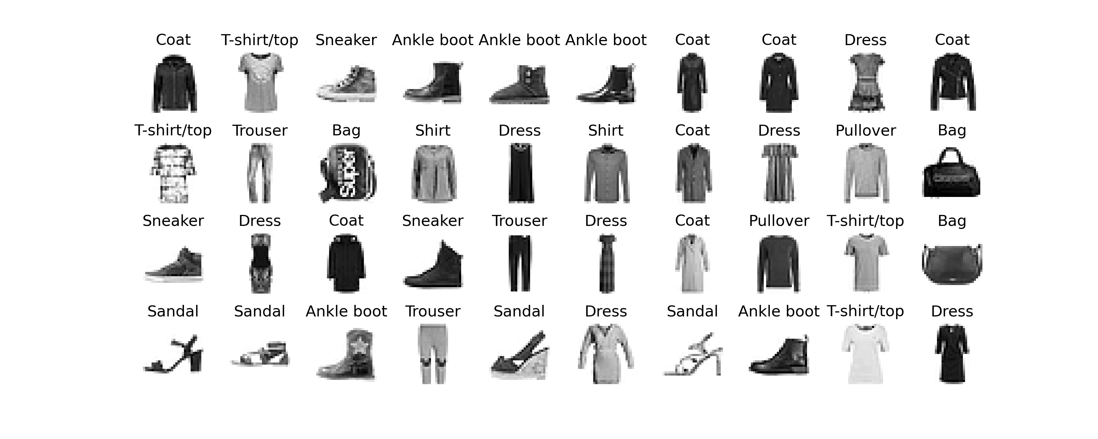
Let’s take a quick look at a sample of the images in the dataset to give us a feel of the complexity of the classification task:

Exponential Learning Rate

The learning rate is arguably the most important hyperparameter. In general, the optimal learning rate is about half of the maximum learning rate (i.e., the learning rate above which the training algorithm diverges). One way to find a good learning rate is to train the model for a few hundred iterations, starting with a very low learning rate (e.g., 1e-5) and gradually increasing it up to a very large value (e.g., 10). This is done by multiplying the learning rate by a constant factor at each iteration. If you plot the loss as a function of the learning rate (using a log scale for the learning rate), you should see it dropping at first. But after a while, the learning rate will be too large, so the loss will shoot back up: the optimal learning rate will be a bit lower than the turning point). You can then reinitialize your model and train it normally using this good learning rate.

Model Building with Keras

We are ready to begin building our MLP with Keras. Here is a classification MLP with two hidden layers:

Let’s go through this code line by line:

• First, we create a Sequential model which is the simplest kind of Keras model for neural networks that are just composed of a single stack of layers connected sequentially.
• Next, we build the first layer and add it to the model. It is a Flatten layer whose purpose is to convert each input image into a 1D array: if it receives input data X, it computes X.reshape(-1, 1). Since it is the first layer of the model, you should specify the input_shape. Alternatively, you could add a keras.layers.InputLayer as the first layer, setting its input_shape=[28,28]
• Next, we add a Dense hidden layer with 300 neurons and specify it to use the ReLU activation function. Each Dense layer manages its own weight matrix, containing all the connection weights between the neurons and their inputs. It also manages a vector of bias terms, one for each neuron.
• Then we add a second Dense hidden layer with 100 neurons, also using the ReLU activation function.
• Finally, we add a Dense output layer with 10 neurons, using the softmax activation function (because we are performing classification with each class being exclusive).

#deep-learning #artificial-neural-network #keras #tensorboard #artificial-intelligence #deep learning