What is Deep Learning?

It’s learning from examples. That’s pretty much the deal.

At a very basic level, Deep Learning is a Machine Learning technique. It teaches a computer to filter inputs through layers to learn how to predict and classify information. Observations can be in the form of images, text, or sound.

The inspiration for Deep Learning is the way that the human brain filters information. Its purpose is to mimic how the human brain works to create some real magic.

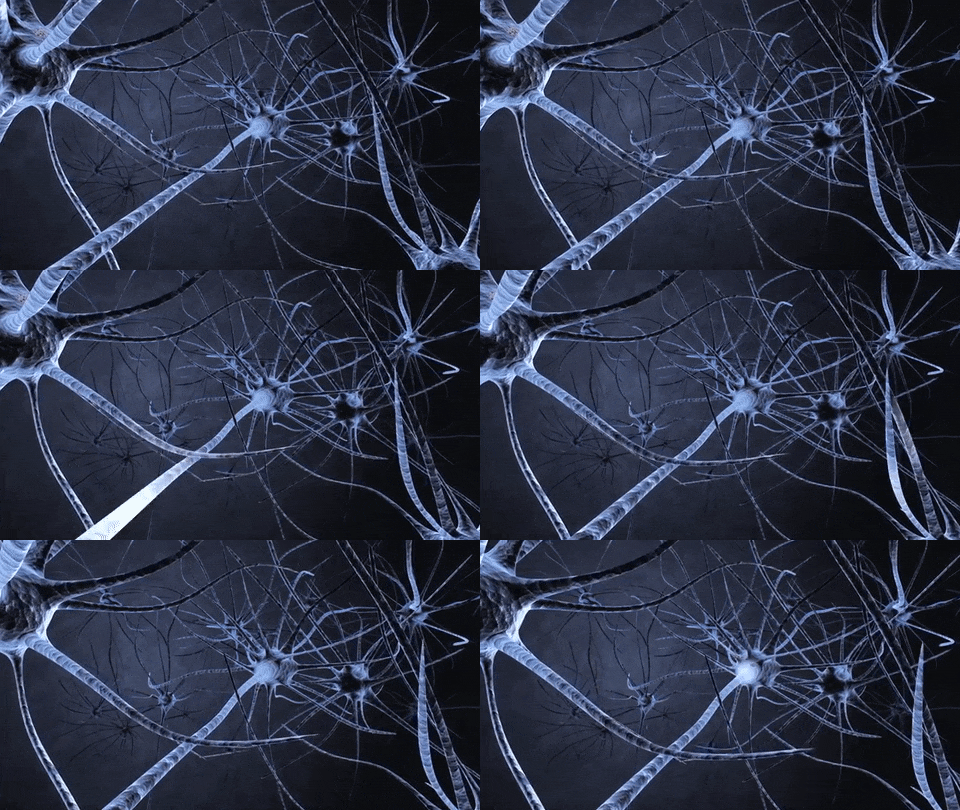
It’s literally an artificial neural network.

In the human brain, there are about 100 billion neurons. Each neuron connects to about 100,000 of its neighbors. We’re kind of recreating that, but in a way and at a level that works for machines.

In our brains, a neuron has a body, dendrites, and an axon. The signal from one neuron travels down the axon and transfers to the dendrites of the next neuron. That connection where the signal passes is called a synapse.

Neurons by themselves are kind of useless. But when you have lots of them, they work together to create some serious magic. That’s the idea behind a deep learning algorithm! You get input from observation and you put your input into one layer. That layer creates an output which in turn becomes the input for the next layer, and so on. This happens over and over until your final output signal!

The neuron (node) gets a signal or signals ( input values), which pass through the neuron. That neuron delivers the output signal.

Think of the input layer as your senses: the things you see, smell, and feel, for example. These are independent variables for one single observation. This information is broken down into numbers and the bits of binary data that a computer can use. You’ll need to either standardize or normalize these variables so that they’re within the same range.

They use many layers of nonlinear processing units for feature extraction and transformation. Each successive layer uses the output of the previous layer for its input. What they learn forms a hierarchy of concepts. In this hierarchy, each level learns to transform its input data into a more and more abstract and composite representation.

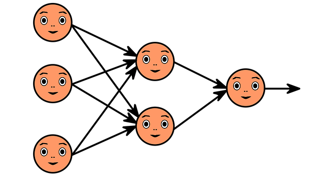
Image by ahmedgad on Pixabay

That means that for an image, for example, the input might be a matrix of pixels. The first layer might encode the edges and compose the pixels. The next layer might compose an arrangement of edges. The next layer might encode a nose and eyes. The next layer might recognize that the image contains a face, and so on.

What happens inside the neuron?

The input node takes in information in a numerical form. The information is presented as an activation value where each node is given a number. The higher the number, the greater the activation.

Based on the connection strength (weights) and transfer function, the activation value passes to the next node. Each of the nodes sums the activation values that it receives (it calculates the weighted sum) and modifies that sum based on its transfer function. Next, it applies an activation function. An activation function is a function that’s applied to this particular neuron. From that, the neuron understands if it needs to pass along a signal or not.

Each of the synapses gets assigned weights, which are crucial to Artificial Neural Networks (ANNs). Weights are how ANNs learn. By adjusting the weights, the ANN decides to what extent signals get passed along. When you’re training your network, you’re deciding how the weights are adjusted.

The activation runs through the network until it reaches the output nodes. The output nodes then give us the information in a way that we can understand. Your network will use a cost function to compare the output and the actual expected output. The model performance is evaluated by the cost function. It’s expressed as the difference between the actual value and the predicted value. There are many different cost functions you can use, you’re looking at what the error you have in your network is. You’re working to minimize loss function. (In essence, the lower the loss function, the closer it is to your desired output). The information goes back, and the neural network begins to learn with the goal of minimizing the cost function by tweaking the weights. This process is called backpropagation.

In forward propagation, information is entered into the input layer and propagates forward through the network to get our output values. We compare the values to our expected results. Next, we calculate the errors and propagate the info backward. This allows us to train the network and update the weights. (Backpropagation allows us to adjust all the weights simultaneously.) During this process, because of the way the algorithm is structured, you’re able to adjust all of the weights simultaneously. This allows you to see which part of the error each of your weights in the neural network is responsible for.

When you’ve adjusted the weights to the optimal level, you’re ready to proceed to the testing phase!

Photo by Yogendra Singh from Pexels

How does an artificial neural network learn?

There are two different approaches to get a program to do what you want. First, there’s the specifically guided and hard-programmed approach. You tell the program exactly what you want it to do. Then there are neural networks. In neural networks, you tell your network the inputs and what you want for the outputs, and then you let it learn on its own.

By allowing the network to learn on its own, you can avoid the necessity of entering in all of the rules. You can create the architecture and then let it go and learn. Once it’s trained up, you can give it a new image and it will be able to distinguish output.

Feedforward and feedback networks

A feedforward network is a network that contains inputs, outputs, and hidden layers. The signals can only travel in one direction (forward). Input data passes into a layer where calculations are performed. Each processing element computes based upon the weighted sum of its inputs. The new values become the new input values that feed the next layer (feed-forward). This continues through all the layers and determines the output. Feedforward networks are often used in, for example, data mining.

A feedback network (for example, a recurrent neural network) has feedback paths. This means that they can have signals traveling in both directions using loops. All possible connections between neurons are allowed. Since loops are present in this type of network, it becomes a non-linear dynamic system which changes continuously until it reaches a state of equilibrium. Feedback networks are often used in optimization problems where the network looks for the best arrangement of interconnected factors.

What is a weighted sum?

Inputs to a neuron can either be features from a training set or outputs from the neurons of a previous layer. Each connection between two neurons has a unique synapse with a unique weight attached. If you want to get from one neuron to the next, you have to travel along the synapse and pay the “toll” (weight). The neuron then applies an activation function to the sum of the weighted inputs from each incoming synapse. It passes the result on to all the neurons in the next layer. When we talk about updating weights in a network, we’re talking about adjusting the weights on these synapses.

A neuron’s input is the sum of weighted outputs from all the neurons in the previous layer. Each input is multiplied by the weight associated with the synapse connecting the input to the current neuron. If there are 3 inputs or neurons in the previous layer, each neuron in the current layer will have 3 distinct weights: one for each synapse.

In a nutshell, the activation function of a node defines the output of that node.

The activation function (or transfer function) translates the input signals to output signals. It maps the output values on a range like 0 to 1 or -1 to 1. It’s an abstraction that represents the rate of action potential firing in the cell. It’s a number that represents the likelihood that the cell will fire. At it’s simplest, the function is binary: yes (the neuron fires) or no (the neuron doesn’t fire). The output can be either 0 or 1 (on/off or yes/no), or it can be anywhere in a range. If you were using a function that maps a range between 0 and 1 to determine the likelihood that an image is a cat, for example, an output of 0.9 would show a 90% probability that your image is, in fact, a cat.

What is an activation function?

In a nutshell, the activation function of a node defines the output of that node.

The activation function (or transfer function) translates the input signals to output signals. It maps the output values on a range like 0 to 1 or -1 to 1. It’s an abstraction that represents the rate of action potential firing in the cell. It’s a number that represents the likelihood that the cell will fire. At it’s simplest, the function is binary: yes (the neuron fires) or no (the neuron doesn’t fire). The output can be either 0 or 1 (on/off or yes/no), or it can be anywhere in a range.

What options do we have? There are many activation functions, but these are the four very common ones:

Threshold function

This is a step function. If the summed value of the input reaches a certain threshold the function passes on 0. If it’s equal to or more than zero, then it would pass on 1. It’s a very rigid, straightforward, yes or no function.

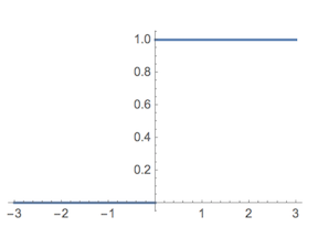
Example threshold function

Sigmoid function

This function is used in logistic regression. Unlike the threshold function, it’s a smooth, gradual progression from 0 to 1. It’s useful in the output layer and is used heavily for linear regression.

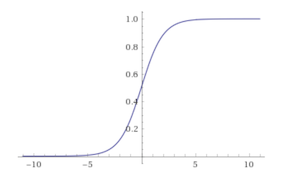
Example sigmoid function

Hyperbolic Tangent Function

This function is very similar to the sigmoid function. But unlike the sigmoid function which goes from 0 to 1, the value goes below zero, from -1 to 1. Even though this isn’t a lot like what happens in a brain, this function gives better results when it comes to training neural networks. Neural networks sometimes get “stuck” during training with the sigmoid function. This happens when there’s a lot of strongly negative input that keeps the output near zero, which messes with the learning process.

Example hyperbolic tangent function (tanh)

Rectifier function

This might be the most popular activation function in the universe of neural networks. It’s the most efficient and biologically plausible. Even though it has a kink, it’s smooth and gradual after the kink at 0. This means, for example, that your output would be either “no” or a percentage of “yes.” This function doesn’t require normalization or other complicated calculations.

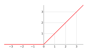
Example rectifier function

What?

So let’s say, for example, your desired value is binary. You’re looking for a “yes” or a “no.” Which activation function do you want to use?

From the above examples, you could use the threshold function or you could go with the sigmoid activation function. The threshold function would give you a “yes” or “no” (1 or 0). The sigmoid function would be able to give you the probability of a yes.

If you were using a sigmoid function to determine how likely it is that an image is a cat, for example, an output of 0.9 would show a 90% probability that your image is, in fact, a cat.

Photo by minanafotos on Pixabay

How do you adjust the weights?

You could use a brute force approach to adjust the weights and test thousands of different combinations. But even with the most simple neural network that has only five input values and a single hidden layer, you’ll wind up with 10⁷⁵ possible combinations.

Running this on the world’s fastest supercomputer would take longer than the universe has existed so far.

Enter gradient descent

But if you go with gradient descent, you can look at the angle of the slope of the weights and find out if it’s positive or negative in order to continue to slope downhill to find the best weights on your quest to reach the global minimum.

If you go with gradient descent, you can look at the angle of the slope of the weights and find out if it’s positive or negative. This allows you to continue to slope downhill to find the best weights on your quest to reach the global minimum.

Photo by RANJAN SIMKHADA from Pexels

Gradient descent is an algorithm for finding the minimum of a function. The analogy you’ll see over and over is that of someone stuck on top of a mountain and trying to get down (find the minima). There’s heavy fog making it impossible to see the path, so she uses gradient descent to get down to the bottom of the mountain. She looks at the steepness of the hill where she is and proceeds down in the direction of the steepest descent. You should assume that the steepness isn’t immediately obvious. Luckily, she has a tool that can measure steepness!

Unfortunately, this tool takes forever.

She wants to use it as infrequently as she can to get down the mountain before dark. The real difficulty is choosing how often she wants to use her tool so she doesn’t go off track.

In this analogy, the person is the algorithm. The steepness of the hill is the slope of the error surface at that point. The direction she goes is the gradient of the error surface at that point. The tool she’s using is differentiation (the slope of the error surface can be calculated by taking the derivative of the squared error function at that point). The rate at which she travels before taking another measurement is the learning rate of the algorithm. It’s not a perfect analogy, but it gives you a good sense of what gradient descent is all about. The machine is learning the gradient, or direction, that the model should take to reduce errors.

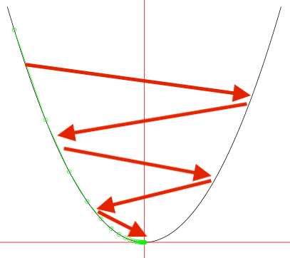
gradient descent (simplified!)

Gradient descent requires the cost function to be convex, but what if it isn’t?

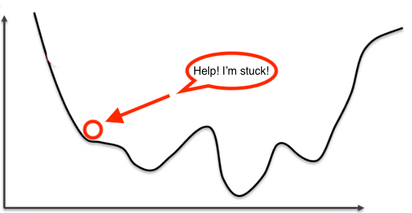
Now what?

Normal gradient descent will get stuck at a local minimum rather than a global minimum, resulting in a subpar network. In normal gradient descent, we take all our rows and plug them into the same neural network, take a look at the weights, and then adjust them. This is called batch gradient descent. In stochastic gradient descent, we take the rows one by one, run the neural network, look at the cost functions, adjust the weights, and then move to the next row. Essentially, you’re adjusting the weights for each row.

Stochastic gradient descent has much higher fluctuations, which allows you to find the global minimum. It’s called “stochastic” because samples are shuffled randomly, instead of as a single group or as they appear in the training set. It looks like it might be slower, but it’s actually faster because it doesn’t have to load all the data into memory and wait while the data is all run together. The main pro for batch gradient descent is that it’s a deterministic algorithm. This means that if you have the same starting weights, every time you run the network you will get the same results. Stochastic gradient descent is always working at random. (You can also run mini-batch gradient descent where you set a number of rows, run that many rows at a time, and then update your weights.)

Many improvements on the basic stochastic gradient descent algorithm have been proposed and used, including implicit updates (ISGD), momentum method, averaged stochastic gradient descent, adaptive gradient algorithm (AdaGrad), root mean square propagation (RMSProp), adaptive moment estimation (Adam), and more.

So here’s a quick walkthrough of training an artificial neural network with stochastic gradient descent:

• Randomly initiate weights to small numbers close to 0
• Input the first observation of your dataset into the input layer, with each feature in one input node.
• Forward propagation — from left to right, the neurons are activated in a way that each neuron’s activation is limited by the weights. You propagate the activations until you get the predicted result.
• Compare the predicted result to the actual result and measure the generated error.
• Backpropagation — from right to left, the error is back propagated. The weights are updated according to how much they are responsible for the error. (The learning rate decides how much we update the weights.)
• Reinforcement learning (repeat steps 1–5 and update the weights after each observation) OR batch learning (repeat steps 1–5, but update the weights only after a batch of observations).
• When the whole training set has passed through the ANN, that is one epoch. Repeat with more epochs.

#deep-learning #machine-learning #artificial-intelligence #data-science