Introduction
Modeling imbalanced data is the major challenge that we face when we train a model. The main objective of my project is to find the best oversampling technique that I will apply on five datasets related to aging-related bug problems. I will use seven machine learning classification models to train the model.
Imbalanced data typically refers to a classification problem where the number of observations per class is not equally distributed; often there will be a large amount of data/observations for one class (referred to as the majority class), and much fewer observations for one or more other classes (referred to as the minority classes).
Data
The datasets I used are related to Aging-Related Bugs (ARBs) that occur in long-running systems due to error conditions caused because of the accumulation of problems such as memory leakage or unreleased files and locks. Aging-Related. Bugs are hard to discover during software testing and also challenging to replicate. Below is the description of each dataset in Table 1.
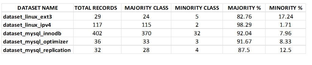
Table 1: Experimental Dataset Description
Balancing Methods Used
1. Class weight
Foremost, I used one of the simplest ways to address the class imbalance that is to simply provide a weight for each class which places more emphasis on the minority classes such that the end result is a classifier that can learn equally from all classes.
2. Oversampling
Secondly, I used three oversampling techniques to remove such an imbalance. For oversampling the minority classes are to increase the number of minority observations until we’ve reached a balanced dataset.
2.1 Random oversampling
It is the most naive method of oversampling. It randomly samples the minority classes and simply duplicates the sampled observations. With this technique, we are artificially reducing the variance of the dataset.
2.2 SMOTE
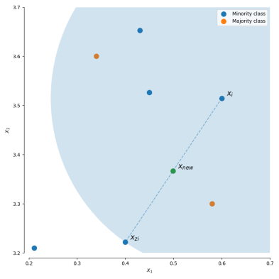
However, we can also use our existing dataset to synthetically generate new data points for the minority classes. Synthetic Minority Over-sampling Technique (SMOTE) is a technique that generates new observations by interpolating between observations in the original dataset.
For a given observation xi, a new (synthetic) observation is generated by interpolating between one of the k-nearest neighbors, xzi.
Xnew = xi+ λ (xzi − xi) xnew = xi + λ (xzi−xi)
where λ is a random number in the range [0,1][0,1]. This interpolation will create a sample on the line between xi and xzi.
2.3 ADASYN
Adaptive Synthetic (ADASYN) sampling is the same as SMOTE, however, the number of samples generated for a given xi is proportional to the number of nearby samples which do not belong to the same class as xi. Thus, ADASYN tends to focus solely on outliers when generating new synthetic training examples.
Classification Models Used
1. **_K Nearest Neighbors — _**Firstly I used a simple classification model that is a KNN classifier. In this model, classification is computed from a simple majority vote of the k nearest neighbors of each point.
**_2. Logistic Regression- _**Second I used Logistic Regression. In this algorithm, the probabilities describing the possible outcomes of a single trial are modeled using a logistic function that is the sigmoid function.
**_3. Naïves Bayes- _**Next I used the Naive Bayes algorithm which is based on Bayes’ theorem with the assumption of independence between every pair of features. Naive Bayes classifiers work well in many real-world situations such as document classification and spam filtering.
**_4. Decision Tree- _**Then I used Decision Tree Classifier. A decision tree produces a sequence of rules that can be used to classify the data. This classifier is simple to understand and visualize and can handle both numerical and categorical data.
#imbalanced-data #classification #comparative-analysis #oversampling #data analysis