Building an Interactive Dictionary, Creating Web Maps using Folium, Building a Website Blocker, Build and Deploy a Website using Flask and Heroku App, Twitter Sentiment Analysis, Scraping data from FIFA.com using BeautifulSoup, Data Collector Web Application using PostgreSQL and Flask, Learn ABC of OpenCV with memes and a little bit of code, Building Financial Graphs using Bokeh …

Master Python through building real-world applications (Part 1): Building an Interactive Dictionary

The internet is a mess and at times, without apt resources, learning a new programming language could be a tedious task. And in that case, the majority of learners give up or they pick something else to play with. So, let me assure you one thing before we start, this is not just any other ‘learn python programming’ post you stumble upon while surfing on the internet. Trust me, it’s not. What we are going to do in this series of 10 posts is to use python to build 10 real-world applications and as we go along, learn other important and necessary tools to master our python skills for Data Science.

What people fail to understand is that learning a programming language is important. No matter how hard it seems, you have to start. So don’t worry if you don’t have any practical experience of programming using python, as long as you know the very basics of python, we are good to go.

The first application we are going to build is a dictionary. An interactive dictionary. I know, I know, it’s easy. But a journey of thousand miles begins with a single step, so you have to take the first step. Now, what the dictionary will do? It will retrieve the definition for the word which user has entered, that’s what dictionaries do, right? In addition to that, if the user has made a typo while entering a word, our program will suggest the closest word saying ‘did you mean this instead?’, and if the word has more than one definition, retrieve all of them. Doesn’t seem that easy now, huh? Let’s find out.

At the end of this article, you are going to feel the same as this man below going to feel after his jump. Because learning or experiencing something new makes us feel motivated and amazing. And that’s what you are going to do today.

Note — In addition to learning how to build applications, pay close attention to how the code is written. Clean code is equally important.

Step 1 — The Data

To know how the dictionary will work, we must understand what data it will use to perform those actions. So, let’s get to it. The Data here is in JSON format. If you already know what JSON is, feel free to skip through the next several lines. However, on the other hand, if you have heard the word JSON for the first time or you need a little refresher, I’ve got you covered. I encourage you to look at the data which we are going to use for a better understanding of the JSON format. You will find the data here and here.

Here is a fun fact, about 2,500,000,000,000,000,000 (2.5 Quintillion) bytes of data is being generated every second, as of 2017. You’ve read it right, every second.
JSON, or JavaScript Object Notation, is a minimal, readable (for both — humans as well as computers)format for structuring data. It mainly has two things, a key and a value associated with the key. Let’s take example from our data only, below is a key/value pair. The key is “abandoned industrial site”, the word and the value is “Site that cannot be used for any purpose, being contaminated by pollutants”, the definition. To understand more about JSON, refer to this article.

"abandoned industrial site": ["Site that cannot be used for any purpose, being contaminated by pollutants."]

Let us start with the code now. First, we import the JSON library, followed by that we use the load method of that library to load our data which is in .json format. The important thing here is that we load data in .json format but it will be stored in “data” variable as python ‘dictionary’. If you are not aware of python dictionaries, think of it as a storage. It is almost the same as a JSON format and it follows the same key-value ritual.

#Import library
import json

#Loading the json data as python dictionary
#Try typing "type(data)" in terminal after executing first two line of this snippet
data = json.load(open("data.json"))

#Function for retriving definition
def retrive_definition(word):
    return data[word]

#Input from user
word_user = input("Enter a word: ")

#Retrive the definition using function and print the result
print(retrive_definition(word_user))

As soon as the data is loaded, let’s create a function which will take the word and will look for the definition of that word in the data. Easy stuff.

Step 2 — Check for non-existing words

Usage of the basic if-else statement will help you check for the non-existing words. If the word is not present in the data, simply let the user know. In our case, it will print “The word doesn’t exist, please double check it.”

#Import library
import json

#Loading the json data as python dictionary
#Try typing "type(data)" in terminal after executing first two line of this snippet
data = json.load(open("dictionary.json"))

#Function for retriving definition
def retrive_definition(word):
    #Check for non existing words
    if word in data:
        return data[word]
    else:
        return ("The word doesn't exist, please double check it.")

#Input from user
word_user = input("Enter a word: ")

#Retrive the definition using function and print the result
print(retrive_definition(word_user))

Step 3 — The case-sensitivity

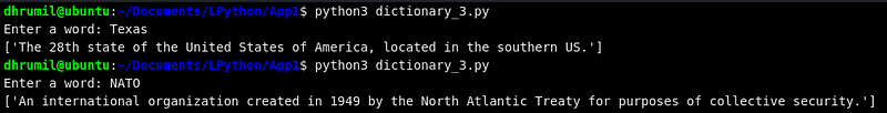
Each user has his or her own way of writing. While some may write in all lower-case, some of them might want to write the same word in title-case, our objective is that the output to the word must remain the same. For example ‘Rain’ and ‘rain’ will give the same output. In order to do that, we are going to convert the word which the user has entered to all lower case because our data has the same format. We will do that with Python’s own lower() method.

Case 1 — To make sure the program returns the definition of words that start with a capital letter (e.g. Delhi, Texas) we will also check for the title case letters in else-if condition.

Case 2 — To make sure the program returns the definition of acronyms (e.g. USA, NATO) we will check for the uppercase as well.

#Import library
import json

#Loading the json data as python dictionary
#Try typing "type(data)" in terminal after executing first two line of this snippet
data = json.load(open("dictionary.json"))

#Function for retriving definition
def retrive_definition(word):
    #Removing the case-sensitivity from the program
    #For example 'Rain' and 'rain' will give same output
    #Converting all letters to lower because out data is in that format
    word = word.lower()

    #Check for non existing words
    #1st elif: To make sure the program return the definition of words that start with a capital letter (e.g. Delhi, Texas)
    #2nd elif: To make sure the program return the definition of acronyms (e.g. USA, NATO)
    if word in data:
        return data[word]
    elif word.title() in data:
        return data[word.title()]
    elif word.upper() in data:
        return data[word.upper()]

#Input from user
word_user = input("Enter a word: ")

#Retrive the definition using function and print the result
print(retrive_definition(word_user))

Your dictionary is ready to serve its basic purpose, retrieve the definition. But let us take it to a step further. Do you find it cool when Google suggest you the correct word while you make a typing error in the search bar?

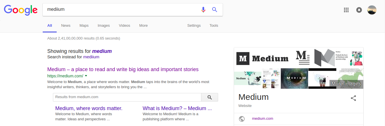
What if we can do the same with our dictionary? Cool, right? Before doing that it Step 5, let’s understand the mechanism behind it in Step 4.

Step 4 — Closest Match

Now, to if the user has made a typo while entering a word, you might want to suggest the closest word and ask them if they want the meaning of this word instead. We can do that with Python’s library difflib. There are two methods to do that, we will understand both and then use the effective one.

Method 1 — Sequence Matcher

Let’s understand this method_._ First, we will import the library and fetch method from it. The SequenceMatcher() function takes total 3 parameters. First one is junk, which means if the word has white spaces or blank lines, in our case that’s none. Second and third parameters are the words between which you want to find similarities. And appended ratio method will give you the result in the number.

#Import library
import json
# This is a python library for 'Text Processing Serveices', as the offcial site suggests.
import difflib
from difflib import SequenceMatcher

#Let's load the same data again
data = json.load(open("dictionary.json"))

#Run a Sequence Matcher
#First parameter is 'Junk' which includes white spaces, blank lines and so onself.
#Second and third parameters are the words you want to find similarities in-between.
#Ratio is used to find how close those two words are in numerical terms
value = SequenceMatcher(None, "rainn", "rain").ratio()

#Print out the value
print(value)

As you can see, the similarity between the word “rainn” and “rain” is 0.89, which is 89%. This is one way to do it. However; there is another method in the same library which fetches close match to the word directly, no numbers involved.

Method 2 — Get Close Matches

The method works as follows, the first parameter is, of course, the word for which you want to find close matches. The second parameter is a list of words to match against. The third one indicates how many matches do you want as an output. And the last one is cut off. Do you remember we got a number in the previous method? 0.89? Cutoff uses that number to know when to stop considering a word as a close match (0.99 being the closest to the word). You can set that according to your criteria.

#Import library
import json
# This is a python library for 'Text Processing Serveices', as the offcial site suggests.
import difflib
from difflib import get_close_matches

#Let's load the same data again
data = json.load(open("dictionary.json"))

#Before you dive in, the basic template of this function is as follows
#get_close_matches(word, posibilities, n=3, cutoff=0.66)
#First parameter is of course the word for which you want to find close matches
#Second is a list of sequences against which to match the word
#[optional]Third is maximum number of close matches
#[optional]where to stop considering a word as a match (0.99 being the closest to word while 0.0 being otherwise)

output = get_close_matches("rain", ["help","mate","rainy"], n=1, cutoff = 0.75)

# Print out output, any guesses?
print(output)

I don’t think I need to explain the output, right? The closest word of all three is rainy, hence [‘rainy’]. If you have come this far, appreciate yourself because you’ve learned the hard part. Now, we just have to insert this into our code to get the output.

Step 5 — Did you mean this instead?

For ease of readability, I’ve just added if-else part of the code. You are familiar with the first two else-if statements, let’s understand the third one. It is first checking for the length of the close matches it got because we can print only if the word has 1 or more close matches. Get close matches function takes the word the user has entered as the first parameter and our whole data set to match against that word. Here, the key is the words in our data and value is their definition, as we learned it earlier. The [0] in return statement indicates the first close match of all matches.

#Check for non existing words
#1st elif: To make sure the program return the definition of words that start with a capital letter (e.g. Delhi, Texas)
#2nd elif: To make sure the program return the definition of acronyms (e.g. USA, NATO)
if word in data:
    return data[word]
elif word.title() in data:
    return data[word.title()]
elif word.upper() in data:
    return data[word.upper()]
#3rd elif: To find a similar word
#-- len > 0 because we can print only when the word has 1 or more close matches
#-- In the return statement, the last [0] represents the first element from the list of close matches
elif len(get_close_matches(word, data.keys())) > 0:
return ("Did you mean %s instead?" % get_close_matches(word, data.keys())[0])

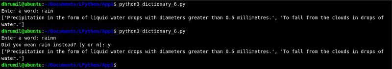
Yes, yes, that’s what I meant. So, what now? you can’t just leave that with a question. If that’s what user meant, you must retrieve the definition of that word. That’s what we are going to do in the next step.

Step 6 — Retrieving the definition

One more input from the user and one more layer of if-else and there it is. The definition of the suggested word.

elif len(get_close_matches(word, data.keys())) > 0:
    action = input("Did you mean %s instead? [y or n]: " % get_close_matches(word, data.keys())[0])
    #-- If the answers is yes, retrive definition of suggested word
    if (action == "y"):
        return data[get_close_matches(word, data.keys())[0]]
    elif (action == "n"):
        return ("The word doesn't exist, yet.")
    else:
return ("We don't understand your entry. Apologies.")

Step 7 — The Icing on the cake

Sure it gets us the definition of rain, but there are square braces and all around it, doesn’t look good huh? Let’s remove them and give it a more cleaner look. The word rain has more than one definition, did you notice? There are several words with more than one definition, so we will iterate through the output of those words having more than one definition and simply print out the ones with a single definition.

#Retrive the definition using function and print the result
output = retrive_definition(word_user)

#If a word has more than one definition, print them recursively
if type(output) == list:
    for item in output:
        print("-",item)
#For words having single definition
else:
print("-",output)

Looks much better, isn’t it? Down below I am attaching the entire code for your reference and feel free to modify and upgrade the code as you like.

The code

#Import library
import json
from difflib import get_close_matches

#Loading the json data as python dictionary
#Try typing "type(data)" in terminal after executing first two line of this snippet
data = json.load(open("data.json"))

#Function for retriving definition
def retrive_definition(word):
    #Removing the case-sensitivity from the program
    #For example 'Rain' and 'rain' will give same output
    #Converting all letters to lower because out data is in that format
    word = word.lower()

    #Check for non existing words
    #1st elif: To make sure the program return the definition of words that start with a capital letter (e.g. Delhi, Texas)
    #2nd elif: To make sure the program return the definition of acronyms (e.g. USA, NATO)
    #3rd elif: To find a similar word
    #-- len > 0 because we can print only when the word has 1 or more close matches
    #-- In the return statement, the last [0] represents the first element from the list of close matches
    if word in data:
        return data[word]
    elif word.title() in data:
        return data[word.title()]
    elif word.upper() in data:
        return data[word.upper()]
    elif len(get_close_matches(word, data.keys())) > 0:
        action = input("Did you mean %s instead? [y or n]: " % get_close_matches(word, data.keys())[0])
        #-- If the answers is yes, retrive definition of suggested word
        if (action == "y"):
            return data[get_close_matches(word, data.keys())[0]]
        elif (action == "n"):
            return ("The word doesn't exist, yet.")
        else:
            return ("We don't understand your entry. Apologies.")

#Input from user
word_user = input("Enter a word: ")

#Retrive the definition using function and print the result
output = retrive_definition(word_user)

#If a word has more than one definition, print them recursively
if type(output) == list:
    for item in output:
        print("-",item)
#For words having single definition
else:
print("-",output)

End Notes

You learn a lot while you are involved in it. Today, you learned about the JSON data, basic functionalities of python, a new library called ‘difflib’ and equally important how to write clean code. Pick your different data set and apply all your skills, because that’s the only way you can become a master in Data Science field.

Happy Learning.

Master Python through building real-world applications (Part 2): Building Web Maps using Folium

Now, in Part 2, we will create a web map using geospatial (pronounce: geo-special) data. On this journey, we will learn how to use folium to create multi-purpose web-maps.

If you went through Part 1 (if you haven’t, I highly recommend you to do so. We will break down the definition into several parts and perform actions step by step, going through each line of the code. Let’s build another cool application.

Step 0 — First things first

We will construct our web map using Python and Folium. You all are aware of Python so let me brief you about Folium. It is basically a Data Visualization library to visualize geospatial data or data that involves coordinates and locations. You will find more about folium on its official project page. Moreover, If you are completely new and don’t know how to install external libraries, I recommend you using ‘pip’, which is a package/library management system, used by most of us.

To install pip, run the following command in your terminal.

#Python 3.x
sudo apt install python3-pip
#Python 2.x
sudo apt install python-pip

Great! You just installed pip and now you are ready to install your first external library. To install folium library, executing following command in your terminal.

pip install folium

Perfect. All the dependencies (fancy term for necessary tools required to run the program, duh) are installed and you are ready to roll.

Step 1 — Creating a Base Map

There is a proverb that says, “Don’t use a lot where a little will do,” while adding my philosophy to that, I came up with, “Start from the basics and don’t use a lot where a little will do.” It is of extreme importance that we start from the basics. Whether it be learning a programming language, or learning how to drive. Basics first. Then add little by little. Always.

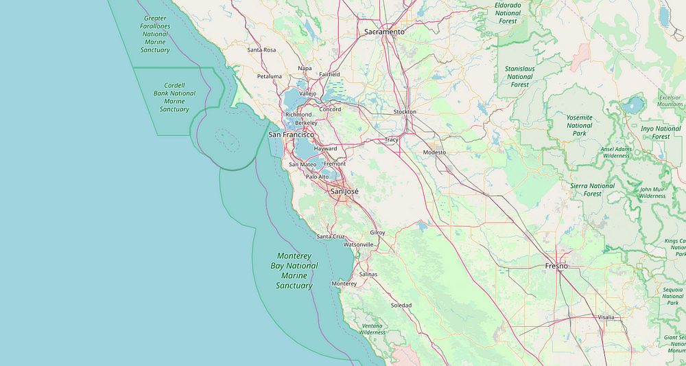
Let’s create a base map. First, we import the library. Now, we create our map with folium.Map which takes the location at which you want your map to start with. You can add additional parameters such as pre-defined zoom and how the map will look like but more on that later. Now you have created your basic map. I believe this is the easiest way to create a map. Save the map, name it as you like and run the code and you will have your first map with folium.

Note — Once you execute the map.save() command, the map is saved in your current working directory. Hence, you have to hit up the file manager, go to the directory you are working in and run the “map1.html” file from there with help of a browser.

#Import Library
import folium

#Create base map
map = folium.Map(location=[37.296933,-121.9574983], zoom_start = 8)

#Save the map
map.save("map1.html")

Step 2 — Add Marker

Marker, a point on the map, is the most important feature of entire map terminology. Let’s add a marker to our map with folium.Marker which also takes the location at which you want to point with some additional parameters such as what popup will display and how the icon will look. Easy stuff. Now the important thing, you see that .add_to(map)? We are adding the marker we created to the map we created earlier. Without this, the marker will be created but won’t be added to our map. Hence, you will see the same blank base map we created earlier.

#Import Library
import folium

#Create base map
map = folium.Map(location=[37.296933,-121.9574983], zoom_start = 8, tiles = "Mapbox bright")

#Add Marker
folium.Marker(location=[37.4074687,-122.086669], popup = "Google HQ", icon=folium.Icon(color = 'gray')).add_to(map)

#Save the map
map.save("map1.html")

Noticed something different in the code? That’s right. We’ve added one more parameter in our base map. Any idea what that is? No? Alright, look at the map.

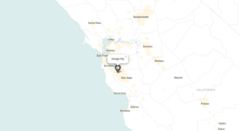
‘tiles’ is a parameter to change the background of the map or to change what data is presented in the map, i.e. streets, mountains, blank map, etc. That’s it, your map is ready with a marker and minimal design. Because less is more.

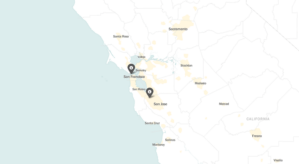
Step 3 — Add Multiple Markers

Adding multiple markers is easy. All you have to do is run a for loop with all the coordinates you want to show. As discussed earlier, the basics, let’s just start with two.

#Import Library
import folium

#Create base map
map = folium.Map(location=[37.296933,-121.9574983], zoom_start = 8, tiles = "Mapbox bright")

#Multiple Markers
for coordinates in [[37.4074687,-122.086669],[37.8199286,-122.4804438]]:
    folium.Marker(location=coordinates, icon=folium.Icon(color = 'green')).add_to(map)


#Save the map
map.save("map1.html")

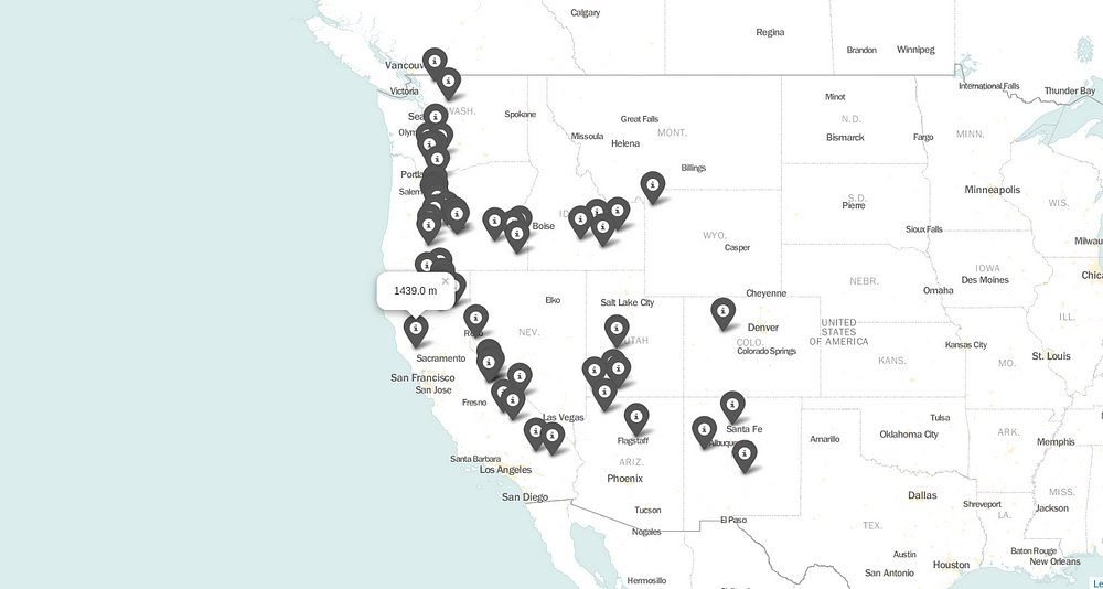
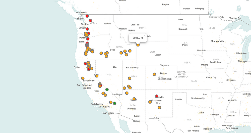
Step 4 — Adding Markers from Data

A pretty neat map you created there. But what if you have 500 markers? Are you going to write them all? Of course not. You must load data and extract relevance data to plot your markers. Here, we have added the data of volcanoes in the United States. You will find the data here.

First, we load data with help of Pandas, which is a commonly used data manipulation library. Refer this page to learn the basics of pandas. The data file includes columns such as the name of the volcano, where it is, elevation, latitude, and longitude. We need latitude and longitude to plot markers and to display a popup, we are going to need elevation. Therefore, we’ll extract it and store it into our variables. Run a for loop and there it is, all the markers with just 2 lines of code.

#Import Library
import folium
import pandas as pd

#Load Data
data = pd.read_csv("Volcanoes_USA.txt")
lat = data['LAT']
lon = data['LON']
elevation = data['ELEV']

#Create base map
map = folium.Map(location=[37.296933,-121.9574983], zoom_start = 5, tiles = "Mapbox bright")

#Plot Markers
for lat, lon, elevation in zip(lat, lon, elevation):
    folium.Marker(location=[lat, lon], popup=str(elevation)+" m", icon=folium.Icon(color = 'gray')).add_to(map)

#Save the map
map.save("map1.html")

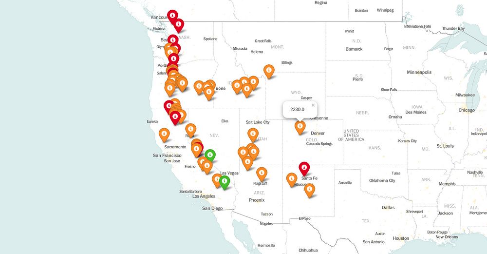
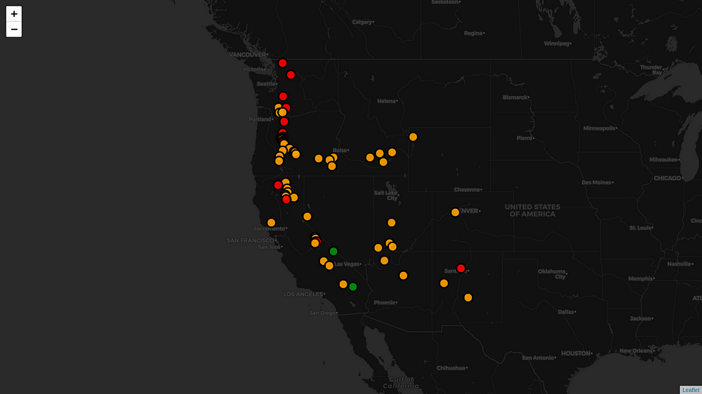
Step 5 — Colors (not by Jason Derulo)

You’ve added all the markers, but they all are in the same color which doesn’t tell much of a story. So, let’s group them by elevation <1000, between 1000 and 3000, and > 3000 and set color to green, orange and red, respectively.

You have to create a function using the simple if-else loops and call it in place of defining a color.

#Import Library
import folium
import pandas as pd

#Load Data
data = pd.read_csv("Volcanoes_USA.txt")
lat = data['LAT']
lon = data['LON']
elevation = data['ELEV']

#Function to change colors
def color_change(elev):
    if(elev < 1000):
        return('green')
    elif(1000 <= elev <3000):
        return('orange')
    else:
        return('red')

#Create base map
map = folium.Map(location=[37.296933,-121.9574983], zoom_start = 5, tiles = "Mapbox bright")

#Plot Markers
for lat, lon, elevation in zip(lat, lon, elevation):
    folium.Marker(location=[lat, lon], popup=str(elevation), icon=folium.Icon(color = color_change(elevation))).add_to(map)

#Save the map
map.save("map1.html")

Step 6 — Change Icons

Let’s admit that the current icon might appear good but it’s not the best. It’s big and feels like we are creating the map in the ’90s. So let’s change them. I hope this is self-explanatory.

#Import Library
import folium
from folium.plugins import MarkerCluster
import pandas as pd

#Load Data
data = pd.read_csv("Volcanoes_USA.txt")
lat = data['LAT']
lon = data['LON']
elevation = data['ELEV']

#Function to change colors
def color_change(elev):
    if(elev < 1000):
        return('green')
    elif(1000 <= elev <3000):
        return('orange')
    else:
        return('red')

#Create base map
map = folium.Map(location=[37.296933,-121.9574983], zoom_start = 5, tiles = "Mapbox bright")

#Plot Markers
for lat, lon, elevation in zip(lat, lon, elevation):
    folium.CircleMarker(location=[lat, lon], radius = 9, popup=str(elevation)+" m", fill_color=color_change(elevation), color="gray", fill_opacity = 0.9).add_to(map)

#Save the map
map.save("map1.html")

Now it looks good. I mean not great, but good. What do we do to make it great? Any ideas? I have got one. Presenting you, The Dark mode. To turn yours into all black, use tiles= “CartoDB dark_matter”

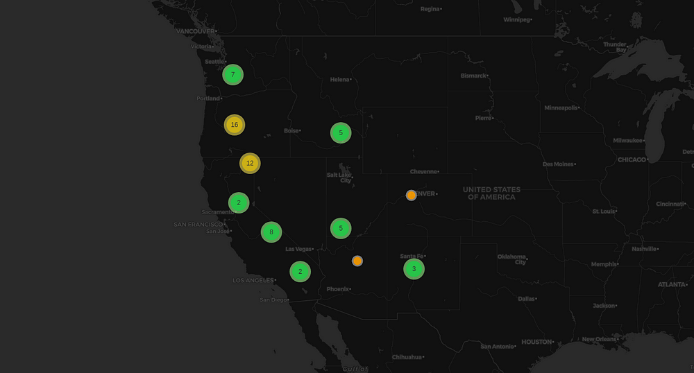
Step 7 — Cluster all Markers

It looks nice but what if you have 300 markers per state? Then it looks all messy. For that, we have to cluster all markers and as we zoom into the map, the cluster unfolds.

In order to do that, first, we have to create a cluster using MarkerCluster method which you will find under the library folium.plugins, and rather than adding all the markers to our map via .add_to(map), we will add them to our cluster via .add_to(name of the cluster), which in our case is .add_to(marker_cluster). Which will look something like shown below. As you zoom in and out of the map, all the clusters will unfold and fold automatically and it will look something like this.

#Import Library
import folium
from folium.plugins import MarkerCluster
import pandas as pd

#Load Data
data = pd.read_csv("Volcanoes_USA.txt")
lat = data['LAT']
lon = data['LON']
elevation = data['ELEV']

#Function to change colors
def color_change(elev):
    if(elev < 1000):
        return('green')
    elif(1000 <= elev <3000):
        return('orange')
    else:
        return('red')

#Create base map
map = folium.Map(location=[37.296933,-121.9574983], zoom_start = 5, tiles = "CartoDB dark_matter")

#Create Cluster
marker_cluster = MarkerCluster().add_to(map)

#Plot Markers and add to 'marker_cluster'
for lat, lon, elevation in zip(lat, lon, elevation):
    folium.CircleMarker(location=[lat, lon], radius = 9, popup=str(elevation)+" m", fill_color=color_change(elevation), color="gray", fill_opacity = 0.9).add_to(marker_cluster)

#Save the map
map.save("map1.html")

Step 8 — One Step Forward

“We are what we repeatedly do,” Aristotle said, “Excellence, therefore, is not an act, but a habit.” Even if you are stuck somewhere in this tutorial, don’t give up. Try again, ask for help, if necessary start from the beginning. Just don’t stop. After all, tenacity is the key to success.

Want to learn more about this? I know. That’s why I’ve added this final map, a choropleth, to help you understand how you can use this library to plot different types of maps with different types of data.

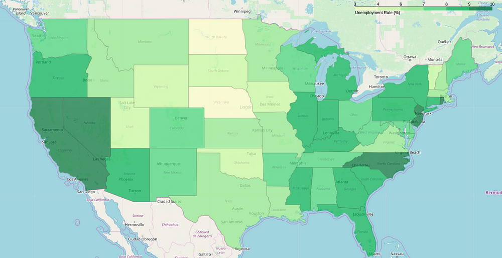
Like what you saw? Want to implement? How about you give it a try by yourself? And if you are stuck somewhere, you can find the entire code on my GitHub repository.

And Of course, End Notes

Appreciate yourself if you have completed both my articles. You have done a great job. While you learned some important aspects of Python programming in the last post, in this one, you have learned what is pip and how to use it, what is folium, what is geospatial data, how to visualize geospatial data using folium, and such things. There’s a lot more in Data Visualization and this is just a tiny part of it. I encourage you to explore more about visualization. My goal was to help you get started, now you have to walk the path.

Happy Learning. And feel free to ask any doubts.

Master Python through building real-world applications (Part 3): Building a Website Blocker in 3 steps

The world is growing rapidly and so does technology. Each day you see something of which you haven’t heard of. But that ain’t a problem. The problem is, how to find the right resources to learn everything in the right order? If you have the same question, you are in for a treat. After this 10 post series, in which you’ll master python, I’m going to create another series on Machine Learning. If you share the same interest as mine, stay tuned.

Here is a fun fact, about 2,500,000,000,000,000,000 (2.5 Quintillion) bytes of data is being generated every second, as of 2017. You’ve read it right, every second.> Here is a fun fact, about 2,500,000,000,000,000,000 (2.5 Quintillion) bytes of data is being generated every second, as of 2017. You’ve read it right, every second.
Before mastering our way to Machine Learning and all the buzzwords people talking about, let’s build a website blocker in Python with basic data structures & file operations to build a strong foundation of core concepts in Python. And to say started from the bottom now we here after 6 months. Maybe. You never know.

Step 1 — Leonardo DiCaprio

Environment. The environment is important. There are mainly three steps in setting up our environment. First, find the path to your hosts file (for windows- C:\Windows\System32\drivers\etc\hosts, and for linux- etc/hosts). If you are good with computers, chances are good that you’ve already played with this file. But if not, hosts file can be used to map hostnames to IP addresses(redirect websites or block them by pointing them to localhost) and is sensitive in any operating system.

Second, we have to define the IP address to which we want to redirect our website, which is localhostin our case. A localhost is that standard hostname given to the machine itself. Commonly represented by the IP address 127.0.0.1. And finally, the list of websites which we want to block.

#Path to the host file
host_path = "/etc/hosts"

#Redirect to local host
redirect = "127.0.0.1"

#Websites to block
website_list = ["www.netflix.com","www.facebook.com"]

Step 2 — Rihanna and Drake

The environment is set. Now, at what time you want to block the websites? It must be work hours, right? But how are we going to define that? We can’t do it manually, or can we? Of course not. Hence, we are going to use Python’s very own date time library to fetch current time whenever the code runs.

We are using the while loop here because it executes the code quickly. Now, in if condition, we are checking if the current time is between 8 AM to 4 PM. While running if it prints Rihanna, you know it’s time to work, work, work work, work. And if it says Drake, have fun its all god’s plan. _time.sleep(5)_ adds five seconds delay. That’s understandable, I believe.

Note — For safety, copy hosts file in your working directory and give the path of that file rather than the original file. Once we have what we need, we will change the path back to the original file.

#Import libraries
import time
from datetime import datetime as dt

#Path to the host file, redirect to local host, list of websits to block
host_path = "/etc/hosts"
redirect = "127.0.0.1"
website_list = ["www.netflix.com","www.facebook.com"]

#Condition
while True:
    #Check for the current time
    if dt(dt.now().year,dt.now().month,dt.now().day,8) < dt.now() < dt(dt.now().year,dt.now().month,dt.now().day,16):
        print("Rihanna")
    else:
        print("Drake")
    time.sleep(5)

Step 3 — Donald Trump

I’m sorry about the PJs but can’t help it. Let’s move to our final step, blocking our websites. We are going to use basic file read/write operations in Python to get this done. This is further divided into two parts. First, we block if the time is working hours and we unblock if the time is fun hours. Let’s do work hours first.

Fetch the current time. Now, to read the content of the file, we need to open it first — basic rules of file operations. We open the file first, then read all the content from that file and store it in our ‘content’ variable, because of course, it is our content. The r+ you see followed by file path, is permission for both, reading and writing, from and to the file. You have opened the file, read the content, so now what? Check if the website is already in the file and if not, put it there. The first part is over, websites from the lists are blocked now. You can see the code in action in the

while True:
    #Check for the current time
    if dt(dt.now().year,dt.now().month,dt.now().day,8) < dt.now() < dt(dt.now().year,dt.now().month,dt.now().day,16):
        print("Rihanna")
        #Open file and read the content
        file = open(host_path,"r+")
        content = file.read()
        for website in website_list:
            if website in content:
                pass
            else:
                #Write the IP of loalhost and name of the website to block
                file.write(redirect + " " + website + "\n")
    else:
        print("Drake")

Its time to Netflix and chill with bae now, so we need to unblock our websites. Basically, we have to remove those websites we have added to the file. In order to achieve that, first, we open the file. Instead of reading the whole file as a string we will read line by line, hence, file.readlines(). The file.seek(0) is used to place the pointer to the starting position of the file. Now the important stuff. Read twice and slowly. The iteration may look complicated to you but it’s not. It is if and for in the same line. website in line checks the first line of hosts file, now which website it is looking for? It comes from the for loop followed by that, w_ebsite in our website list_. In a nutshell, the meaning of the entire line is, if our website from website list is not there in the line of host file, append/print that line. If the line has our website, then ignore that line. I hope this clears up the meaning because it is important. And there it is, removing the websites from the list.

else:
        print("Drake")
        #Open hosts file and read content from it- line by line
        file = open(host_path,'r+')
        content = file.readlines()
        #Take back pointer to starting of the file from the end of file
        file.seek(0)
        for line in content:
            #Please check explaination for this line
            if not any(website in line for website in website_list):
                file.write(line)
            file.truncate()
    time.sleep(5)

Almost there

You did a great work creating the website blocker but you don’t want to execute the code every day to block websites, right? That’s why we will use a task scheduler to perform this job. We are going to use Cron Job Scheduler (it is pre-installed in the operating system, you don’t have to install anything). Just Open cron table with sudo permission and parameter -e.

add the path of our main file followed by a command — @reboot

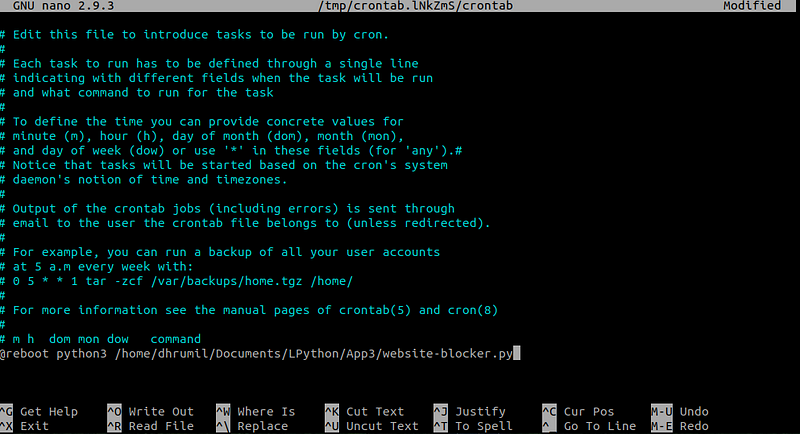
It is done now. You have successfully blocked websites on our list. Reboot your computer to see the changes and if you have any problems regarding anything in the article, hit me up. My email and Twitter DMs are always open. Also, happy to hear any suggestions and feedbacks.

End Notes

Website blockers are common these days and you can easily find them in your browser’s app store as an extension. But how many of us really know how those things work? Scant people. Knowing how such things works is important. Find the entire code for this application as well as other application on my GitHub profile. Kudos to you for learning this. And until next part, Happy Learning.

Master Python through building real-world applications (Part 4): Build and Deploy a Website using Flask and Heroku App

Every once in a while, there comes a new programming language and along with that great community to support that. Python has been around for a while now so it is safe for me to say that Python is not a language, it is a religion. Do you want to print hello world? It’s there. Make database applications? There. Make GUI based applications? Yup. Visualization? Checked. Complex Machine Learning algorithms? Python’s got you covered. If you think of something that is programmable, you can do that with Python. Though there is one field where Python is underrated, and it is at the back-end of web development. But soon enough, it will change too. And we will take the first step to know more about it.

They all build websites using just HTML and CSS, what’s new in that? In this article, we are going to build a website using Python and Flask. And once we have our website, we will deploy it on Heroku’s web servers so that everyone on the internet can see what you’ve created. Also, this might help you in your future ML or DL developments. Got all freshen up? Because this might take a while. Let’s do it.

Step 1 — Understanding Flask

Flask is a microframework for Web Development. By micro, it means it is very basic in its nature. No external tools or libraries come pre-installed with it. Flask is commonly used with MongoDB, which gives it more control over databases and history. I think that’s enough introduction. What we actually want to see is how it works, right? So let’s get to it. But before we do that, we need to clear one fundamental concept of Flask framework, which is Routes.

Routes are nothing but a specific path. As Abhinav explains, let’s imagine you’re visiting apple.com and want to go to the Mac section at apple.com/mac/. How do Apple’s servers know to serve you the specific page that shows the details about Mac devices It is most likely because they have a web app running on a server that knows when someone looks up apple.comand goes to the /mac/ section of the website, handle that request and send some pages back, mostly the index file in that folder.

Step 2 — Creating a Basic Website

Creating a basic website using Python and Flask is like walking in the park. You just write 5 lines of code and you are there.

1. First, from the flask framework, import Flask class.
2. Create a variable to store your flask object instance or in other words, your flask application. The parameter __name__ here assigns a name to the app, by default it is __main__
3. The route, as we discussed, is a path or URL where you’ll view your website. In this case, it is set at the root of our directory.
4. Then we create a function. This function defines what our web page will do. For now, we have just printed out hello world.
5. Running the script. If your app has the name __main__ then the script will execute, as simple as that. But, if you are calling this script from another piece of code, our __name__ parameter from step 2 will assign or app the name of our file which is script1 , therefore the script will not execute.

#Import dependencies
from flask import Flask

#Create instance of Flask App
app = Flask(__name__)

#Define Route
@app.route("/")

#Content
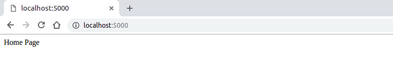
def home():
    return("Home Page")

#Running and Controlling the script
if (__name__ =="__main__"):
    app.run(debug=True)

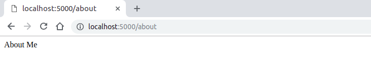
Still confused about routes? Look at the next snippet to get a clear picture. All websites have About me page, right? So let’s add the same to our website as well. We have two different routes that serve two different pages.

#Import dependencies
from flask import Flask

#Create instance of Flask App
app = Flask(__name__)

#Define Route and Contant of that page
@app.route("/")
def home():
    return("Home Page")

#Define 2nd Route and Content
@app.route("/about")
def about():
    return("About Me")

#Running and Controlling the script
if (__name__ =="__main__"):
    app.run(debug=True)

Step 3 — HTML and CSS

The website we just created is not something you enjoy watching. So, what do we do to make it more appealing? HTML and CSS, of course. They are best suited for this task. If you know your way around web development, you can create a new .html file from scratch. But if you don’t know how to do that, there are plenty of templates available out on the internet, find the one that suits you.

Now, rather than just returning simply text, we are going to return specific HTML pages that we’ve created. To do that, we have to import another class that is render_template. Then in our content function, we have to return render_template("file.html") to see specific HTML file on that route.

#Import dependencies
from flask import Flask, render_template

#Create instance of Flask App
app = Flask(__name__)

#Define Route and Contant of that page
@app.route("/")
def home():
    return render_template("home.html")

#Define 2nd Route and Content
@app.route("/blog")
def about():
    return render_template("blog.html")

#Running and Controlling the script
if (__name__ =="__main__"):
    app.run(debug=True)

**For HTML **— All .html files that you are calling, must reside in a folder named templates in your working directory.

For CSS — For all .css and .js files, you have to create a folder called static and in the folder add sub-folder called css, now put your .css files here.

Appreciate yourself, you have what it takes to reach your goal. We have created our website and it is running perfectly fine on the localhost. Hence, we will take a step further. Your website will be visible to the whole internet. That’s right. We will take it live by deploying it to the cloud. We will be using the Heroku cloud, it allows you to deploy python applications in their cloud, for free. But before that, let’s set up a virtual environment in our local system.

Step 4 — Setting up Virtual Environment

You must be thinking, now what the heck is this virtual environment, right? I thought the same. But don’t worry, I got you. Virtual environment will help us isolate our development environment and package installations from the rest of our system. So, what we install in our virtual environment will never show up in our actual system. Pretty neat, huh. Let’s set it up.

1. First, from the flask framework, import Flask class.
2. Create a variable to store your flask object instance or in other words, your flask application. The parameter __name__ here assigns a name to the app, by default it is __main__
3. The route, as we discussed, is a path or URL where you’ll view your website. In this case, it is set at the root of our directory.
4. Then we create a function. This function defines what our web page will do. For now, we have just printed out hello world.
5. Running the script. If your app has the name __main__ then the script will execute, as simple as that. But, if you are calling this script from another piece of code, our __name__ parameter from step 2 will assign or app the name of our file which is script1 , therefore the script will not execute.

Step 5 — Deploying the Website to a Live Server

Okay, let’s get back to our website. Deploying a python website is not easy just like we do with HTML or PHP file, dragging and dropping using an FTP client. Therefore, we are going to do everything in order, please be patient and follow each step carefully.

Step 5.1 — Creating a Heroku Account

Create an account for Heroku by following this link.

Step 5.2 — Installing the required tools

First in line is git, we will use git to upload our files to the live server. If you are new to git, follow this article to get yourself familiar with it. And to install git, fire up your command line and type the following,

sudo apt install git-all

If you are setting up the git first time, you may want to configure it with your name and email address by typing following, individually.

git config --global user.name "John Doe"
git config --global user.email johndoe@example.com

Second in line is, Heroku CLI , think of it as Heroku’s own git. To install,

sudo snap install --classic heroku

Alrighty. We have what we need. Let’s move further.

Step 5.3 — Setting up Heroku from the command line

We have to set up Heroku where our application is. So, let’s head towards the folder where our main script is, and log in with Heroku credentials. You’ll be asked to press any key to log in and you’ll be redirected to the browser. Once you provide your credentials and successfully log in, your command window should look like this.

Now, we have to create our application. Make sure to name it properly because it is your domain name followed by herokuapp.com., i.e. hello.herokuapp.com I tried my first name but it’s already taken. So, I had to go with dhrumilp and there it is.

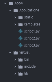
Step 5.4 — Creating the required files (total 3)

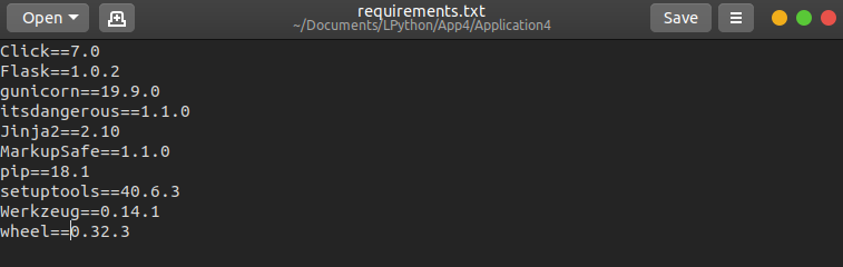
**1.** **requirements.txt —**It contains the list of dependencies (libraries) that we want Heroku to install in their python installation so that our app works fine. To do that, first head into the virtual environment we created earlier, install gunicorn with help of pip, it is a Python Web Server. Once done, type pip list to display all the dependencies we have and type pip list > requirements.txt to create a text file with that list. Just what we wanted. You might see the text file in your directory, move it to where our python file is.

Important Note — Please use pip freeze > requirements.txt instead and make sure that your requirements file looks like mine shown below, otherwise, Heroku won’t accept it and will throw an error.

**2.** Procfile — This file doesn’t have any extension. And it contains the name of the server & name of the app. Create a file and name it to Procfile and type the following into the file,

web: gunicorn mainscript:app

Here, gunicorn is the server we used. mainscript is the name of the python file and app is the name of application we gave while creating the instance of flask class (see the code snippet of step 2), so if you have different names, please change them.

**3.** **runtime.txt —**It contains which version of Python you want to use. In this file, write,

python-3.7.0

I am using Python 3.x that’s why I have used this runtime. If you are using Python 2.x, use python-2.7.15 instead. Perfect, we have what we need. Now, we just have to upload everything.

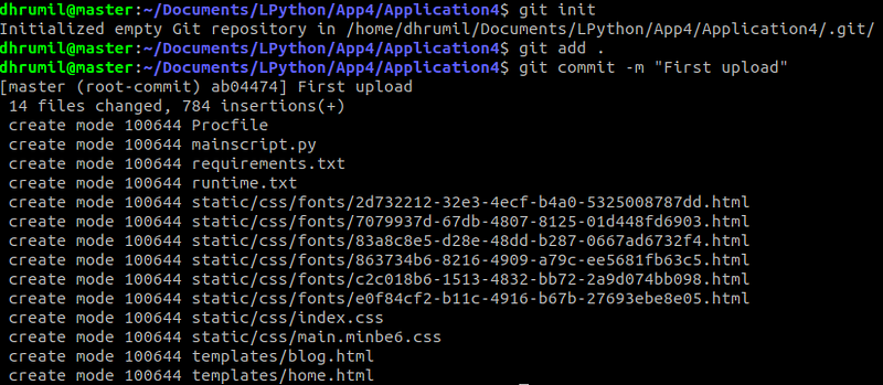
Step 5.5 — Uploading Everything

Alright. Rather than explaining everything one-by-one, I’ll explain each line with a comment. You have to execute each line individually.

#Make sure you are in the same folder as your main python file
#Make sure you are logged in to heroku, if not
heroku login
#Initialize git to upload all the files
git init
#add all the files(it is a period at the end which means all)
git add .
#Now, commit to the server
git commit -m "First upload"
#Call your app that you created
heroku git:remote --app dhrumilp
#Push everything to master branch
git push heroku master

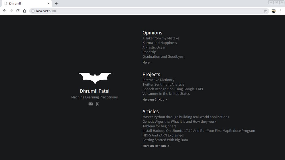
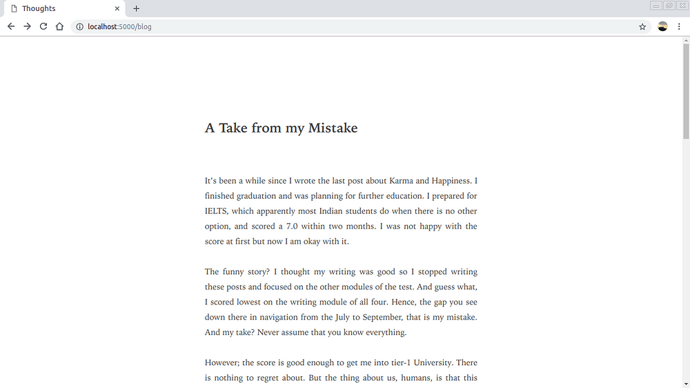
And done. Uffffffff. Congratulations if you have come this far. My app is live at dhrumilp.herokuapp.com , feel free to check it out.

Step 6 — And Finally, Maintaining the Website

We don’t usually update our websites every day, but when we do, we want those changes to be reflected upon the live website. So whenever you change something in your website, you have to upload those changes to the Heroku app. To do that, we just have to repeat what we just did.

#Make sure you are in the same folder as your main python file
#First log in to Heroku
heroku login
#Fetch your app
heroku git:remote --app dhrumilp
#Use git to upload all your changes (don't forget the period)
git add .
git commit -m "Changes"
git push heroku master

And just like that, you maintain your live website which we built using Python and Flask and Heroku and all the other apps/libraries/dependencies that helped us.

End Notes

Holy smoke that was a lot of work but we did it. Web development using Python is underrated right now but there are people and companies who understand its worth. Also, not for just websites, you can use this method to deploy your python apps on the web. Now that you’ve created front end, how about we collect data from our web application? I’ve created a post where we collect data using Flask and PostgreSQL. Check it out here.

Master Python through building real-world applications (Part 5): Twitter Sentiment Analysis in 3 Minutes

In this part, we are going to create a Python script that uses Twitter to understand how people are feeling about a topic that we choose. We will use Natural Language Processing library TextBlob and write merely 15 lines of code to get this done. So why Twitter? Because whether we like it or not, people around the world put thousands of reactions and opinions on every topic they might encounter, every day, every second. Before diving into the code, let’s first understand the basic mechanism behind sentiment analysis.

How Sentiment Analysis Works

1. First, from the flask framework, import Flask class.
2. Create a variable to store your flask object instance or in other words, your flask application. The parameter __name__ here assigns a name to the app, by default it is __main__
3. The route, as we discussed, is a path or URL where you’ll view your website. In this case, it is set at the root of our directory.
4. Then we create a function. This function defines what our web page will do. For now, we have just printed out hello world.
5. Running the script. If your app has the name __main__ then the script will execute, as simple as that. But, if you are calling this script from another piece of code, our __name__ parameter from step 2 will assign or app the name of our file which is script1 , therefore the script will not execute.

That’s that. That is how it works. Now that you know how it works theoretically, let’s learn how it works practically.

Step 1 — Getting things ready

We only need two libraries to perform sentiment analysis using Twitter. First is tweepy, a Python library for accessing Twitter API. And the second is textblob, which is a library for processing textual data. Also, it provides simple API for diving into common natural language processing (NLP) tasks such as part-of-speech tagging, noun phrase extraction, sentiment analysis, and more.

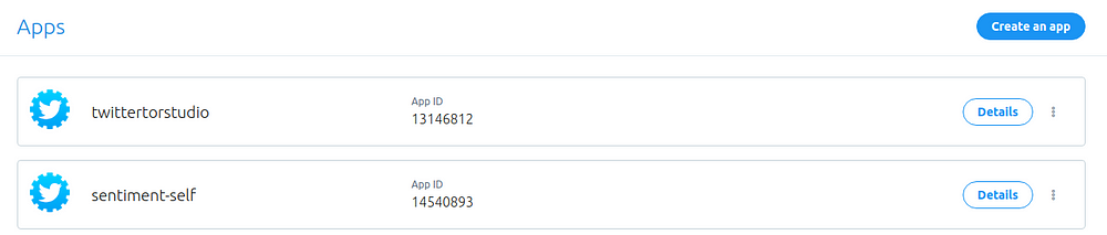
To use Twitter’s data, you’ll have to go to the Developer Apps page on Twitter and create an application. Creating an application will give you your own set of keys that we will use later in this article.

#Import libraries
import tweepy
from textblob import TextBlob

#Create your app from apps.twitter.com and fill your keys and tokens
consumer_key = '3KFL*************'
consumer_secret = 'yltO********************'
access_token = '3014895**************'
access_token_secret = 'w7rZ********************'

Step 2 — Authenticate your application

As soon as you have the keys and tokens, the next thing to do is authenticate yourself. 0AuthHandler takes the authentication keys. Access tokens define the permission — Read, Write or Both. Once that is complete, provide that to tweepy’s API method and it’s done.

#Authenticate your application
auth = tweepy.OAuthHandler(consumer_key, consumer_secret)
auth.set_access_token(access_token, access_token_secret)
api = tweepy.API(auth)

Step 3 — Sentiment Analysis

With help of our authenticated account (api), we can search for specific keywords for which we need sentiment analysis. Once the keyword is set and tweets are called, we will handle tweets with textblob.

First, we will print out the latest tweets related to our keyword. After that, we will use textblob to find the sentiment of that particular tweet and print that out too. Let’s see what Apple’s CEO Tim Cook has to say.

#Search for tweets
public_tweets = api.search('Tim Cook')
for tweet in public_tweets:
    #Print tweets
    print(tweet.text)
    #Use textblob to fetch sentiment of the tweet
    analysis = TextBlob(tweet.text)
    print(analysis.sentiment)
    print('\n')

As you see the output, It prints out series of tweets and with that its sentiment analysis. The important thing to note here is, Polarity indicates how positive or negative the tweet is ( -1 < sentiment < 1) and subjectivity measure how much of a personal opinion is there in the text.

End Notes

I tried to keep this post concise as Sentiment Analysis is an important aspect in Data Science and information overload might set you off even without starting. There are enormous applications where Sentiment Analysis is used, I encourage you to explore them. You can reach out to me via email, Twitter or even Linkedin if you have any doubts. Also, the entire code can be found on my GitHub repository. Happy Learning.

Master Python through building real-world applications (Part 6): Scraping data from FIFA.com using BeautifulSoup

Most people think data science is about cool machine learning algorithms and self-driving cars. Let me tell you something, it’s not. Almost 80% of the time you are searching and cleaning the data, and if successful, remaining 20% in those cool stuff you see upfront. “**Find data and play with it”**is most repeated advice a new-comer in data science could get_._ I am sure you have read it somewhere too, right? But, what if you really want to work on some project but the data you want is not there on the internet? No one is teaching what will you do then, do they?

Here is a fun fact, about 2,500,000,000,000,000,000 (2.5 Quintillion) bytes of data is being generated every second, as of 2017. You’ve read it right, every second.> Here is a fun fact, about 2,500,000,000,000,000,000 (2.5 Quintillion) bytes of data is being generated every second, as of 2017. You’ve read it right, every second.> Here is a fun fact, about 2,500,000,000,000,000,000 (2.5 Quintillion) bytes of data is being generated every second, as of 2017. You’ve read it right, every second.
Data that you are going to need might not always be there in plain sight. But the good news is, it is there. Hidden in the web pages. You just have to crawl through those pages to extract it. That’s what Web Scraping is. And today, we are going to build a web scraper using Python and BeautifulSoup (a library) to scrap data of FIFA World Cup 2018. The data includes individual player’s information and statistics of the whole world cup. Interesting enough? Then what are we waiting for? Let’s shoot.

Step 0 — Understanding What Data to Scrap

I was looking for data to scrap and was jumping from one page to another. 10 minutes later I was on fifa.com, perfect places exist guys. As soon as I was there, I directed myself towards ‘players’ section to find some useful data. And I got some. Now, all we need to do is download this page via Python and scrap data from it.When I say download the page, I mean the HTML code of that page and not any other way around. Let’s first know how to download the page.

Step 1 — Loading the Web page in Python

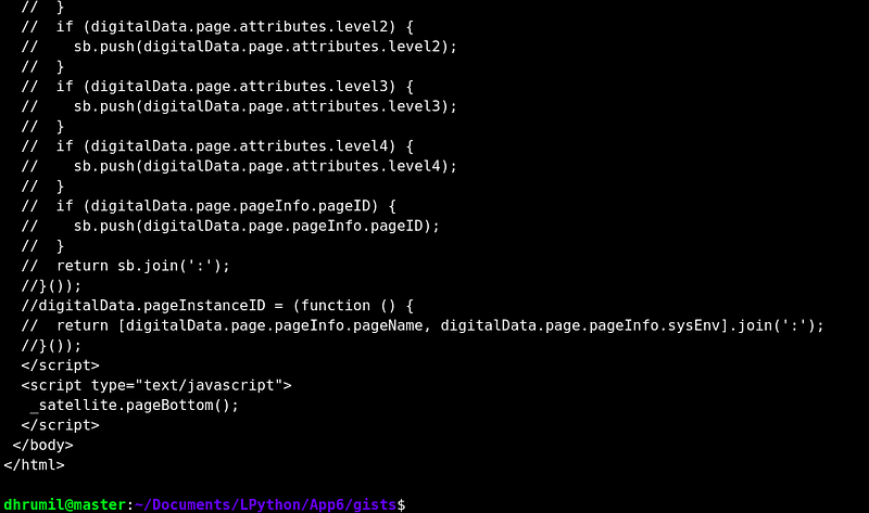
I am sure you have seen this screen at least once before coming here. If not, you can see this (the code of the webpage) by clicking right click anywhere on that page and selecting Inspect Element. I am putting it here so that when we load the page in python, you’ll know we have loaded the right page.

#Import libraries
import requests
from bs4 import BeautifulSoup

#Request URL
page = requests.get("https://www.fifa.com/worldcup/players.html")

#Fetch webpage
soup = BeautifulSoup(page.content,"html.parser")
print(soup.prettify())

requestsThe first thing we are going to need to scrap the page is to download the page. We are going to do that with Python’s requests library.

BeautifulSoup

We will use this library to parse the HTML page we’ve just downloaded. In other words, we’ll extract the data we need.

With requests.get you first get the webpage by passing the URL. Now, we create an instance of BeautifulSoup. We will print that instance to check whether the web page loaded correctly or not. Adding .prettify() makes code cleaner so that it is readable to humans. As you can see, our page has loaded correctly. Now we can scrape data from it.

Step 2 — First Player

Here is a fun fact, about 2,500,000,000,000,000,000 (2.5 Quintillion) bytes of data is being generated every second, as of 2017. You’ve read it right, every second.> Here is a fun fact, about 2,500,000,000,000,000,000 (2.5 Quintillion) bytes of data is being generated every second, as of 2017. You’ve read it right, every second.
Scraping is easiest when the web developer has done his part diligently because we will use HTML attributes to know what exact data to scrape. Not sure what? Stay with me for a minute and you will. Look at the image below.

What did you see? I am on Ronaldo’s profile page. Correct. I have opened the code of that page. Right. But what am I pointing at? His name. Because I want to scrape that name. So, I check in the code how it is written. Turns out, there is a separate division and a separate class name. That’s what we are going to use. Now take a look at the code.

#Import libraries
import requests
from bs4 import BeautifulSoup

#Request URL
page = requests.get("https://www.fifa.com/worldcup/players/player/201200/profile.html")

#Fetch webpage
soup = BeautifulSoup(page.content,"html.parser")

#Scraping Data
name = soup.find("div",{"class":"fi-p__name"})
print(name)

We have requested the page where Ronaldo’s profile resides. Created an instance. Now, with find method of BeautifulSoup, we will find what we need. We need div but there are a lot of div in the code, which one do you need specifically? We need the one where the class name is fi-p__name only. Because in that division, name of the player is written. And voila, we got it.

Simplifying the Output

#Import libraries
import requests
from bs4 import BeautifulSoup

#Request URL
page = requests.get("https://www.fifa.com/worldcup/players/player/201200/profile.html")

#Fetch webpage
soup = BeautifulSoup(page.content,"html.parser")

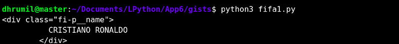
#Scraping Data
name = soup.find("div",{"class":"fi-p__name"}).text.replace("\n","").strip()
print(name)

We can’t store the data in the format we got right? We need it in the text format. That’s why we have added .text at the end. And this is what it looks like.

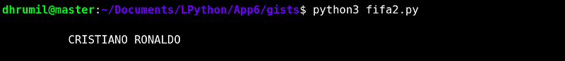
Still not cool, we have several “\n” there. We got to remove them as well. So we will replace them with nothing. And we will have something like this,

One more thing, removing preceding and following spaces, for that, .strip() and the final output looks like this.

There we have it. We have fetched the name of one player. With the same thing, we will fetch other details which you saw on the web page. Like, height, country, role, and goals.

Step 3 — All Data of First Player

#Import libraries
import requests
from bs4 import BeautifulSoup

#Request URL
page = requests.get("https://www.fifa.com/worldcup/players/player/201200/profile.html")

#Fetch webpage
soup = BeautifulSoup(page.content,"html.parser")

#Scraping Data
#Name #Country #Role #Age #Height #International Caps #International Goals
player_name = soup.find("div",{"class":"fi-p__name"}).text.replace("\n","").strip()
player_country = soup.find("div",{"class":"fi-p__country"}).text.replace("\n","").strip()
player_role = soup.find("div",{"class":"fi-p__role"}).text.replace("\n","").strip()
player_age = soup.find("div",{"class":"fi-p__profile-number__number"}).text.replace("\n","").strip()
player_height = soup.find_all("div",{"class":"fi-p__profile-number__number"})[1].text.replace("\n","").strip()
player_int_caps = soup.find_all("div",{"class":"fi-p__profile-number__number"})[2].text.replace("\n","").strip()
player_int_goals = soup.find_all("div",{"class":"fi-p__profile-number__number"})[3].text.replace("\n","").strip()

print(player_name,"\n",player_country,"\n",player_role,"\n",player_age,"years \n",player_height,"\n",player_int_caps,"caps \n",player_int_goals,"goals")

Each parameter has its own class. Easy for us. While height, caps, and goals don’t, huh. No worries. We will use find_all method and then we will print each with the index number in their order. Tada, we made it simple too. The output looks something like this.

https://cdn-images-1.medium.com/max/800/1*rZt_XXfNLEstnuTbwn2eIg.png

Step 4 — All Data of All 736 Players

That’s the data of one player we got, how about others? All player’s profiles are on different web pages. We have to have it all with just one script and not individual scripts for each player. What are we going to do now? Find a pattern, so that we can fetch all URL’s at the same time.

As you can see, the URL of the Ronaldo’s profile is, [[https://fifa.com/worldcup/players/player/201200/profile.html](https://fifa.com/worldcup/players/player/201200/profile.html)](https://fifa.com/worldcup/players/player/201200/profile.html](https://fifa.com/worldcup/players/player/201200/profile.html) "https://fifa.com/worldcup/players/player/201200/profile.html](https://fifa.com/worldcup/players/player/201200/profile.html)") , do you see something which might be common for all? Yes, there is. The player id (for Ronaldo — 201200) might be unique for all of them. So, before scraping all other data, we have to scrape player IDs. Just like we scraped the name, but this time we will run a loop.

Now while going through the source code, I found this link where all the Player IDs are mentioned. That’s why I have taken this page to scrape those IDs.

#Import libraries
import requests
from bs4 import BeautifulSoup
import pandas

#Empty list to store data
id_list = []

#Fetching URL
request = requests.get("https://www.fifa.com/worldcup/players/_libraries/byposition/[id]/_players-list")
soup = BeautifulSoup(request.content,"html.parser")

#Iterate to find all IDs
for ids in range(0,736):
    all = soup.find_all("a","fi-p--link")[ids]
    id_list.append(all['data-player-id'])

#Data Frame to store scrapped data
df = pandas.DataFrame({
"Ids":id_list
})
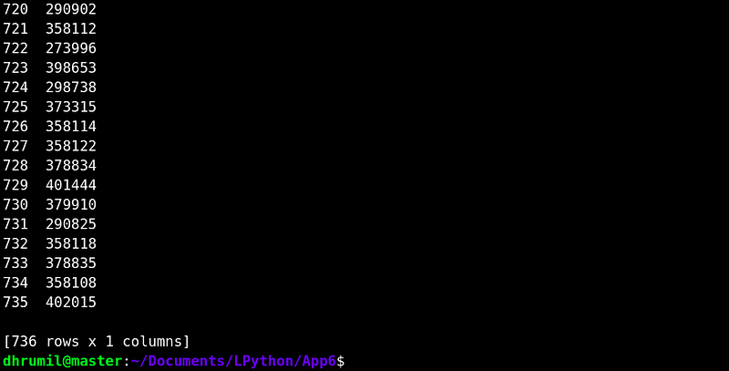
df.to_csv('player_ids.csv', index = False)
print(df,"\n Success")

I checked the website, there were total 736 players, hence, running a loop to for the same. Here, in place of div there is a , the anchor tag. But the functionality remains the same — Searching and finding our class. We are creating an empty list at the beginning, and then appending the IDs to that list in each iteration. In the end, we will create a data frame to store those IDs and export them to .CSV file.

Fetching All Data of All Players

Now that we have the IDs, and know how to fetch each parameter, we just have to pass those IDs and run all through the iteration. Take a look.

#Import libraries
import requests
from bs4 import BeautifulSoup
import pandas
from collections import OrderedDict

#Fetch data of Player's ID
player_ids = pandas.read_csv("player_ids.csv")
ids = player_ids["Ids"]

#Prive a base url and an empty list
base_url = "https://www.fifa.com/worldcup/players/player/"
player_list = []

#Iterate to scrap data of players from fifa.com
for pages in ids:
    #Using OrderedDict instead of Dict (See explaination)
    d=OrderedDict()
    #Fetching URLs one by one
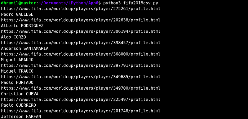
    print(base_url+str(pages)+"/profile.html")
    request = requests.get(base_url+str(pages)+"/profile.html")
    #Data processing
    content = request.content
    soup = BeautifulSoup(content,"html.parser")
    #Scraping Data
    #Name #Country #Role #Age #Height #International Caps #International Goals
    d['Name'] = soup.find("div",{"class":"fi-p__name"}).text.replace("\n","").strip()
    print(d['Name'])
    d['Country'] = soup.find("div",{"class":"fi-p__country"}).text.replace("\n","").strip()
    d['Role'] = soup.find("div",{"class":"fi-p__role"}).text.replace("\n","").strip()
    d['Age'] = soup.find("div",{"class":"fi-p__profile-number__number"}).text.replace("\n","").strip()
    d['Height(cm)'] = soup.find_all("div",{"class":"fi-p__profile-number__number"})[1].text.replace("\n","").strip()
    d['International Caps'] = soup.find_all("div",{"class":"fi-p__profile-number__number"})[2].text.replace("\n","").strip()
    d['International Goals'] = soup.find_all("div",{"class":"fi-p__profile-number__number"})[3].text.replace("\n","").strip()

#Append dictionary to list
player_list.append(d)
#Create a pandas DataFrame to store data and save it to .csv
df = pandas.DataFrame(player_list)
df.to_csv('Players_info.csv', index = False)
print("Success \n")

We have created a base URL, so when we iterate through each ID, only ID in the URL will change, and we will get data from all the URLs. One more thing is, rather than lists, we are using dictionaries because there are multiple parameters. And specifically Ordered Dictionary because we want the same order as we fetch the data and not the sorted one. Append dictionary to list and create a data frame. Save the Data to CSV and there you have it. I’ve printed out only the name of the player while running the script because that way I can be sure that data is fetched correctly.

We have done it. If you’re here with me too, you are a great learner. I have uploaded the data to my Kaggle profile, do check that out.

Step 5 — The Statistics

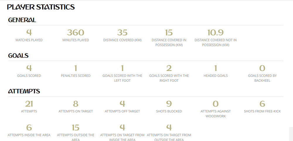
We ain’t gonna stop now, are we? On the player’s page, I found these statistics of the entire world cup, and again my brain was like, “looks like we have another page to scrap.” I spent the entire day scraping data, and I scraped these statistics as well. But hey, you now know all you need to know about web scraping with Python and BeautifulSoup, why don’t you try that by yourself? Oh wait, I have an idea.

Try scraping this by yourself. If you can’t somehow, I have it on my GitHub repository. But (there is always a but), that code has a flaw in that too. Find that flaw or complete this scraping by yourself and open a pull request on the repository. If you have the correct solution I will shoutout your GitHub/Medium profile in the next article I write. Or maybe something else that can help you in ML journey.

I am aware that the code can be optimized in many ways, but for now, our focus is on learning. No matter how your program performs in terms of time and space complexity, if you have the correct solution, we are on the right path. You are learning that’s what is important for now, we will catch up on those things later on.

Endnotes

Today, you have learned about two new libraries and how to use them to download web page and scrap data from those pages. Isn’t that great? You’ll have the edge over your competitors in the interviews if you just have this one extra skill. If you have any doubts, feel free to reach out to me by Email, Twitter or LinkedIn. Any feedback and suggestions are welcome too. Once again check scraped data on my Kaggle profile and submit your solution to my GitHub repository. Read other parts of this series from the links below. Happy Learning.

P.S. If you are from FIFA and reading this, this data I scraped is just for educational purposes and not to breach any of your Data Policies. Don’t sue me.

Master Python through building real-world applications (Part 7): Data Collector Web App with PostgreSQL and Flask

Working with database and queries can be pretty daunting to some, or maybe most of us. Perhaps, I have lost 100 readers by now just because there’s PostgreSQL written in the subtitle. But as you are here, I want you to know that it is an important thing to learn and I will make sure that it is like walking in the park for you. To do that, before we go any further, I want you to read the quoted text. Twice.

Here is a fun fact, about 2,500,000,000,000,000,000 (2.5 Quintillion) bytes of data is being generated every second, as of 2017. You’ve read it right, every second.> Here is a fun fact, about 2,500,000,000,000,000,000 (2.5 Quintillion) bytes of data is being generated every second, as of 2017. You’ve read it right, every second.
I, my self, don’t really enjoy it, but as Robin Sharma said, doing things that we don’t like doing is something that sets us apart from the herd. In this part, we are going to create a website that collects data the user has entered (created using flask) and store it to our database (PostgreSQL). Also, we will make it live so this can work in real time.

Important Note — I have already covered a detailed post Part 4 of this series where we create a web app using Flask and make it live using the Heroku app. Therefore, I will primarily focus on the back end in this article. If you haven’t read that post yet, going quickly through it would be a great idea as you’ll know how to set up the front end, virtual environment, and how to make the application live. Go, I’ll wait for you here.

Alright, everybody on the same page? Let’s begin.

Step 1 — Setting Up Front End

As discussed earlier, we will focus on the back end mainly. But that doesn’t mean we will abandon everything else. I will briefly discuss everything so that it will serve as a refresher for learners following this series from the beginning.

Flask is a micro-framework for web development and is often used while working with the database. We will create a webpage from which we can get the user input. Creating a website with Flask is easy stuff. Look at the code below.

#Import dependencies
from flask import Flask, render_template

#Create instance of Flask App
app = Flask(__name__)

#Define Route and Contant of that page
@app.route("/")
def index():
    return render_template("index.html")

#Define 2nd Route and Content
@app.route("/success", methods = ['POST'])
def success():
    return render_template("success.html")

#Running and Controlling the script
if (__name__ =="__main__"):
    app.run(debug=True)

I know you have gone through Part 4 so you have the idea of how this thing works. The only thing new here is, methods = ['POST'] that’s because we are sending data to the server. Also, make sure to set up the virtual environment for this application as well ( Step 4 in Part 4).

I have downloaded a template and modified to get data of height, weight, sex, and shoe size of the user. You must be thinking why? Taking height, weight is cool but why shoe size? Right? You will know at the end. So the front end looks something like this. It’s up to you how you design your front end.

Step 2— Setting Up Back End

2.1 Create a PostgreSQL Database

To create and store data, we are going to need a database management system. Hence, we are using PostgreSQL for it. If you are on a Windows or Mac machine, there are installers available on the official website and if you are on a Linux machine, find the pgAdmin III app from the Ubuntu Software (16.04 or later). However, if you are using Ubuntu 15.10 or earlier (which I am sure you are not), follow the first answer on this Stack Exchange page to install it manually (we have already created our virtual environment so do the needful apart from that).

Create User

Once you have installed pgAdmin 3, create a user and set a password for that by typing following. Where the first ‘postgres’ is the username and second ‘postgres’ is the database name.

Connect to the localhost server

Open pgAdmin3 and from ‘file’ on the left top corner, select add server. You will see the screen same as mine. Fill it out with your username and password.

As you can see there we have postgres database we created while creating a user. Right click on the ‘databases’ to create a new database to store our data. I have created one which reads Data Collector. That’s the coolest name I thought of. Sorry. So now we have our dataset, we have to create columns (table) in which the data will be stored.

2.2 Connecting Database and Creating Table

SQLAlchemy will help us connect to our database and psycopg is the PostgreSQL wrapper for Python. We don’t have to dwell into that, let’s just install those two libraries and move on with our code.

pip3 install flask_sqlalchemy
pip3 install psycopg2
#Import dependencies
from flask import Flask, render_template
from flask.ext.sqlalchemy import SQLAlchemy

#Create instance of Flask App
app = Flask(__name__)

#Connect to the Database
app.config['SQLALCHEMY_DATABASE_URI']='postgresql://postgres:postgres1@localhost/DataCollector'
db = SQLAlchemy(app)

class Data(db.Model):
    #create a table
    __tablename__ = "data"
    id = db.Column(db.Integer, primary_key = True)
    height = db.Column(db.Integer)
    weight = db.Column(db.Integer)
    shoesize = db.Column(db.Integer)
    sex = db.Column(db.String)

    def __init__(self, height, weight, shoesize, sex):
        self.height = height
        self.weight = weight
        self.shoesize = shoesize
        self.sex = sex

#Define Route and Contant of that page
@app.route("/")
def index():
    return render_template("index.html")

#Define 2nd Route and Content
@app.route("/success", methods = ['POST'])
def success():
    return render_template("success.html")

#Running and Controlling the script
if (__name__ =="__main__"):
    app.run(debug=True)

We have to configure our app with username, password, and database name. After postgresql:// the first is username then a colon and then password. And at last, that’s our database. Once done, we then have to create an instance of SQLAlchemy.

Then comes our class. Object-Oriented Programming to the rescue. If you are not aware of the OOP concepts, here is a good article for you. With help of our instance, we create a model. In which we define table name and all the column names for which we want user input. We don’t want to run the whole code because it is incomplete, therefore we will run this model manually. Go to your app directory, **fire up python console (simply type python)**, and type the following.

from app import db
db.create_all()

As you can see, we have our table and all our columns ready to store data. All we have to do now is write 3 lines of actual code to get things done.

2.3 Store Data to the Database

#Import dependencies
from flask import Flask, render_template, request
from flask_sqlalchemy import SQLAlchemy

#Create instance of Flask App
app = Flask(__name__)

#Connect to the Database
app.config['SQLALCHEMY_DATABASE_URI']='postgresql://postgres:postgres1@localhost/DataCollector'
db = SQLAlchemy(app)

class Data(db.Model):
    #create a table
    __tablename__ = "data"
    id = db.Column(db.Integer, primary_key = True)
    height = db.Column(db.Integer)
    weight = db.Column(db.Integer)
    shoesize = db.Column(db.Integer)
    sex = db.Column(db.String)

    def __init__(self, height, weight, shoesize, sex):
        self.height = height
        self.weight = weight
        self.shoesize = shoesize
        self.sex = sex

#Define Route and Contant of that page
@app.route("/")
def index():
    return render_template("index.html")

#Define 2nd Route and Content
@app.route("/success", methods = ['POST'])
def success():
    if(request.method == 'POST'):
        height_ = request.form["height"]
        weight_ = request.form["weight"]
        shoesize_ = request.form["shoesize"]
        sex_ = request.form["sex"]
        data = Data(height_,weight_,shoesize_,sex_)
        db.session.add(data)
        db.session.commit()
        return render_template("success.html")

#Running and Controlling the script
if (__name__ =="__main__"):
    app.run(debug=True)

As it will check the method is POST, if it is, it will save data user has entered to the variables. Now we have to create a session, add data to the database and commit. There we have it. Done.

Step 3— Deploy the Web App to a Live Server

You already know how to create 3 required files and make your web app live on Heroku App as discussed in Part 4. To make this web app live, first, you just have to repeat the process. Once the web app is live, we now have to create a database on Heroku server and provide that link in our main script in place of localhost. To do that, log in to your Heroku CLI and create a database by typing following command. Where ‘dataforml’ is the name of my app.

Note — Make your app live first and then perform these actions.

heroku addons:create heroku-postgresql:hobby-dev --app dataforml

Type heroku config --app dataforml to see the URI of your database and print it to your main script (See the code below, line 9). Now, one final step. Just like we created the table in our local host, we have to create it on Heroku. So, open Python shell on Heroku by typing following,

heroku run python
from (name of your main file) import db
db.create_all()
exit()

And there it is. Your web data collector app up and running. This is how my final file looks like after configuring the Heroku database (line 9).

#Import dependencies
from flask import Flask, render_template, request
from flask_sqlalchemy import SQLAlchemy

#Create instance of Flask App
app = Flask(__name__)

#Connect to the Database
app.config['SQLALCHEMY_DATABASE_URI']='postgres://qlypyonycmvmjc:4d216baa0889e5e1cf70f59ba26f9fa25e6abc2b6c86d952a489b6c3ef7bf452@ec2-23-23-184-76.compute-1.amazonaws.com:5432/d8cvi73sj545ot?sslmode=require'
db = SQLAlchemy(app)

class Data(db.Model):
    #create a table
    __tablename__ = "data"
    id = db.Column(db.Integer, primary_key = True)
    height = db.Column(db.Integer)
    weight = db.Column(db.Integer)
    shoesize = db.Column(db.Integer)
    sex = db.Column(db.String)

    def __init__(self, height, weight, shoesize, sex):
        self.height = height
        self.weight = weight
        self.shoesize = shoesize
        self.sex = sex

#Define Route and Contant of that page
@app.route("/")
def index():
    return render_template("index.html")

#Define 2nd Route and Content
@app.route("/success", methods = ['POST'])
def success():
    if(request.method == 'POST'):
        height_ = request.form["height"]
        weight_ = request.form["weight"]
        shoesize_ = request.form["shoesize"]
        sex_ = request.form["sex"]
        data = Data(height_,weight_,shoesize_,sex_)
        db.session.add(data)
        db.session.commit()
        return render_template("success.html")

#Running and Controlling the script
if (__name__ =="__main__"):
    app.run(debug=True)

How to know the data is stored correctly? To check the data, you can open the dashboard on Heroku.com or type the following in your command line,

heroku pg:psql --app dataforml

It will fire up a command line query writing, run select * from data and you will see all your recorded data here. Cool huh?

Final Words

Because there are many small processes are involved in the back end, covering them all is a difficult task. But I think I’ve covered all that is necessary. And about the data, I am training a gender classifier which classifies the gender based on height, weight, and shoe size. My web app is currently live at DataForML.herokuapp.com and it will take a minute to respond, I hope you will provide your input. You can find all the codes (including front end) on my GitHub repository.

Master Python through building real-world applications (Part 8): Learn ABC of OpenCV while building a Face and Motion detector

There is no doubt that Data Science (in general) is the next big thing and these numbers are proof that Data Scientists love Python. And as we all know, numbers don’t lie. Learning some aspects of Data Science and Python together would be a great idea, right? That’s why we are going to focus on the real world application of Data Science using Python for our remaining three applications.

We will start with Computer Vision. It’s not that we are going to build a system for a self-driving car but you’ll learn a number of things today. The road ahead is a little long, so take a break if you need, this is the time. Back? Let’s go. Now install OpenCV — called Open Source Computer Vision Library— by typing the following command and let’s get started.

pip3 install opencv-python --user

Step 1— Load, Display, and Resize Images

Let’s start with baby steps. As Computer Vision is all about images and videos, we will first perform several operations such as loading, displaying, resizing and writing (save) on any image you like. Since meme is the language that we all understand, why don’t we start with this one?

#Import OpenCV library
import cv2

#Loading Image
#Where, 0 = Grayscale and 1 = RGB
our_image = cv2.imread("0.jpeg",0)

#Type of 'our_image' object
print(type(our_image))
print(our_image.shape, "\n")
print(our_image)

First, as always, we import our library. Then with theimread function of OpenCV, we load the image. The second parameter is either 0 (grayscale), 1 (RGB), or -1 (transparency capabilities). Size of our image is 675x1200. The important thing to note here is that the image is loaded as a numpy N-dimensional array. Look at the output, our image has broad white borders (hover over the image) that’s why the pixel values of all four corners would be 255. Why don’t you check out how the array looks when you use 1 instead of 0?

Resize the Image

Resizing the image is easy. We call cv2.resize function and pass our image as the first argument and our desired size as the second argument. Now to display and save the image, we need to understand the following,

1. First, from the flask framework, import Flask class.
2. Create a variable to store your flask object instance or in other words, your flask application. The parameter __name__ here assigns a name to the app, by default it is __main__
3. The route, as we discussed, is a path or URL where you’ll view your website. In this case, it is set at the root of our directory.
4. Then we create a function. This function defines what our web page will do. For now, we have just printed out hello world.
5. Running the script. If your app has the name __main__ then the script will execute, as simple as that. But, if you are calling this script from another piece of code, our __name__ parameter from step 2 will assign or app the name of our file which is script1 , therefore the script will not execute.

#Import OpenCV library
import cv2

#Loading Image
#Where, 0 = Grayscale and 1 = RGB
our_image = cv2.imread("0.jpeg",0)

#Resizing our image
resized_image = cv2.resize(our_image, (600,188))

#Show Imaage in a window
cv2.imshow("Memes",resized_image)
cv2.imwrite("generated_memes.jpg", resized_image)
cv2.waitKey(0)
cv2.destroyAllWindows()

Step 2— Batch Image Resizing

We are not robots, we are humans. We are smart. We won’t resize each image individually. Instead, we will make use of our brains. Take a look, you’ll be like, “ah, it’s that easy?”

Glob here finds all the images with .jpg extension within the same directory.

#Import libraries
import cv2
import glob

#Find all images with .jpeg extension
images = glob.glob("*.jpg")

for img in images:
    #Loading all images one by one
    our_image = cv2.imread(img,0)

    #Resizing all image
    resized_image = cv2.resize(our_image, (300,300))

    #Show Imaage in a window
    cv2.imshow("Batch",resized_image)
    cv2.imwrite("resized_"+img, resized_image)
    cv2.waitKey(500)
    cv2.destroyAllWindows()

Step 3— Face Detection in Images

I am sure you’ve seen laptop screens where there’s a webcam on, recording a video in a tiny frame, and there’s a green square around the person’s face, right? Yes. Face detection. Ever wondered how they do it? Wonder no more. Only two things here are new than the previous code. First is Cascade Classifier and second is Detect Multi-Scale. Let’s understand what those two does.

cv2.CascadeClassifier() — A Cascade Classifier is a classifier trained with several hundred “positive” sample views of a particular object (i.e. face) and arbitrary “negative” images of the same size. After the classifier is trained, it can be applied to a new image and detect the object in question. In our case, we will use the pre-trained ‘frontface’ classifier to detect the face in our image. Read more about it here and find more classifiers to play with here.

face_cascade.detectMultiScale() — It is used to know the exact location of the face in the image. We have two new parameters here, let’s learn what they are and why they are useful. scaleFactor resize the image so that when given larger or smaller faces, it is detectable by the algorithm.

Using a small step for resizing, for example, 1.05 which means you reduce the size by 5 %, you increase the chance of a matching size with the model for detection is found. Read this for more information on scale factor.

minNeighbors is the parameter which will affect the quality of the detected faces. Higher value results in fewer detections but with higher quality.

#Importing Library
import cv2

#Load Cascade
face_cascade = cv2.CascadeClassifier("haarcascade_frontface_default.xml")

#Load image
our_image_color = cv2.imread("elon-weed.jpg")
our_image_gray = cv2.cvtColor(our_image_color,cv2.COLOR_BGR2GRAY)

#detect face
faces = face_cascade.detectMultiScale(our_image_gray,
scaleFactor = 1.05,
minNeighbors = 5
)

#Print out type and values of object faces 
print(type(faces))
print(faces)

If you’ll look at the output, there are four values in the faces object. If you see these four values, that means it has detected a face. But where? The answer is those four values. First two are241 & 153, which is the x & y coordinates of the starting point of the detected face (top left corner). Followed by that is 206 & 206, which is witdth & height of the area of the detected face, respectively.

Now that we know where’s the face in the image, we have to mark it so that it is distinguishable. We will use cv2.rectangle() to mark the rectangle. Let’s understand the parameters. First is the image, of course. Second is the starting point of our detected face as we discussed. Third is lowest down corner. And in last, there is the thickness of the rectangle.

#Importing Library
import cv2

#Load Cascade
face_cascade = cv2.CascadeClassifier("haarcascade_frontface_default.xml")

#Load image
our_image_color = cv2.imread("elon-weed.jpg")
our_image_gray = cv2.cvtColor(our_image_color,cv2.COLOR_BGR2GRAY)

#Detect face
faces = face_cascade.detectMultiScale(our_image_gray,
scaleFactor = 1.05,
minNeighbors = 5
)

#Draw a rectangle around face
for x, y, w, h in faces:
    our_image_rect = cv2.rectangle(our_image_color, (x,y), (x+w,y+h), (0,255,0), 3)

#Show Image
cv2.imshow("Face Detection", our_image_rect)
cv2.waitKey(0)
cv2.destroyAllWindows

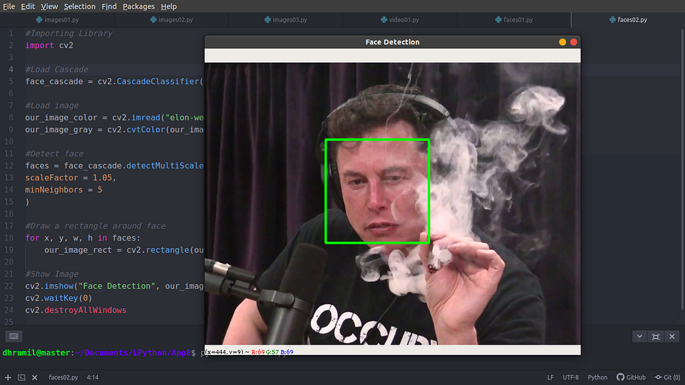
That’s it. There we have detected Elon Musk smoking Marijuana (and feeling nothing, maybe)

Step 4— Capturing Video

Let’s take a step forward by capturing a video. A video is nothing but a collection of images or as some would say a collection of frames. It’s the same thing. As you can see, we are calling the VideoCapture method of the cv2 library and passing 0 which means capturing from the webcam of your own laptop. frame prints the array of the first image/frame of the video.

#Import Library
import cv2

#Capture Video
our_video = cv2.VideoCapture(0)

#Check if loaded correctly
check, frame = our_video.read()
print(check, "\n", frame)

#release video
our_video.release()

But what if we want to show the actual video that our webcam is taking? We have to use the cv2.imshow method and iterate just like we did in batch image resizing.

#Import Library
import cv2

#Capture Video
our_video = cv2.VideoCapture(0)

while True:
    #Check if loaded correctly
    check, frame = our_video.read()
    print(check, "\n", frame)

    #Show the captured frame of video
    cv2.imshow("Capturing", frame)

    #Set q=quit
    key = cv2.waitKey(1)
    if(key == ord('q')):
        break

our_video.release()
cv2.destroyAllWindows

Here, waitKey(1) means it is taking frames every 1 millisecond. And when you’ll type q it will break the loop and stop capturing the video. Here is how I look while the webcam is on.

I know, I know, I look funny facepalm You can laugh but also make sure you see how the frames change, rapidly. Now that we know how to capture video, let’s learn how to detect objects in real-time, including faces.

Step 5— Motion Detector

Let us first understand theoretically how it works and then we will move towards the code. If you don’t understand something, keep one reading, once you are at the end of the step, everything will make sense.

Why a motion detector?

To be honest, it is easiest to start with. Also, it’s useful in some scenarios. For example, if you want to monitor your baby or your dog (whichever is more important to you. Kidding, it’s the dog of course) while you are away. It has two steps in that. First is detect objects in real time and record time when the object is entering and exiting the frame.

First — Object Detection

1. First, from the flask framework, import Flask class.
2. Create a variable to store your flask object instance or in other words, your flask application. The parameter __name__ here assigns a name to the app, by default it is __main__
3. The route, as we discussed, is a path or URL where you’ll view your website. In this case, it is set at the root of our directory.
4. Then we create a function. This function defines what our web page will do. For now, we have just printed out hello world.
5. Running the script. If your app has the name __main__ then the script will execute, as simple as that. But, if you are calling this script from another piece of code, our __name__ parameter from step 2 will assign or app the name of our file which is script1 , therefore the script will not execute.

3. And then there is a more enhanced version of the delta frame which is the threshold frame. If the difference between the previous frame and this frame is more than, let’s say, 100 intensity, convert those pixels to white. As you can see, my face is in white pixels while the background is black.

4. Basically, that’s how we detect if an object is moving or not. We find the contours (points which moved) of the white image and the area of the contour is more than 500 pixels, then we will consider this as a moving object. And mark those objects with a rectangle.

Let’s look at the code and comments and see how it works.

#Import Library
import cv2

#First frame
first_frame = None

#Capture Video
our_video = cv2.VideoCapture(0)

while True:
    #Check if loaded correctly
    check, frame = our_video.read()

    #Conver to Gray
    our_frame_gray = cv2.cvtColor(frame, cv2.COLOR_BGR2GRAY)
    our_frame_gray = cv2.GaussianBlur(our_frame_gray,(21,21),0)

    #Set first frame
    if first_frame is None:
        first_frame=our_frame_gray
        continue

    #Delta frame
    #Compare first frame to current frame
    delta_frame = cv2.absdiff(first_frame, our_frame_gray)

    #Thresold frame
    threshold_frame = cv2.threshold(delta_frame, 30, 255, cv2.THRESH_BINARY)[1]
    threshold_frame = cv2.dilate(threshold_frame, None, iterations=2)

    #Contours
    cnts, hierarchy = cv2.findContours(threshold_frame.copy(), cv2.RETR_EXTERNAL, cv2.CHAIN_APPROX_SIMPLE)

    #Draw rectangle for moving objects
    for contour in cnts:
        if cv2.contourArea(contour) < 500:
            continue
        x, y, w, h = cv2.boundingRect(contour)
        cv2.rectangle(frame, (x,y), (x+w,y+h), (0,255,0), 3)

    #Show the captured frame of video
    cv2.imshow("First Frame", first_frame)
    cv2.imshow("Capturing first ", our_frame_gray)
    cv2.imshow("Delta Frame", delta_frame)
    cv2.imshow("Threshold Frame", threshold_frame)
    cv2.imshow("Detecting objects", frame)

    #Set q=quit
    key = cv2.waitKey(1)
    if(key == ord('q')):
        break

our_video.release()
cv2.destroyAllWindows

Second — Recording Motion Time

We’ll assume we are monitoring a dog. We have got a camera setup where he usually sits. Now, we will record the time to know how many times he was out of his spot to mess up with the house.

To do that, we first have to define points when the object is entering into the frame and exiting the frame. We will create an object called status and we will set it equal to 0 and 1 (line 20 and 47, respectively).

#Import Library
import cv2
from datetime import datetime
import pandas

#First frame
first_frame = None
status_list = [None, None]
times=[]
df=pandas.DataFrame(columns= ["Start","End"])

#Capture Video
our_video = cv2.VideoCapture(0)

while True:
    #Check if loaded correctly
    check, frame = our_video.read()

    #For motion time
    status = 0

    #Conver to Gray
    our_frame_gray = cv2.cvtColor(frame, cv2.COLOR_BGR2GRAY)
    our_frame_gray = cv2.GaussianBlur(our_frame_gray,(21,21),0)

    #Set first frame
    if first_frame is None:
        first_frame=our_frame_gray
        continue


    #Delta frame
    #Compare first frame to current frame
    delta_frame = cv2.absdiff(first_frame, our_frame_gray)

    #Thresold frame
    threshold_frame = cv2.threshold(delta_frame, 30, 255, cv2.THRESH_BINARY)[1]
    threshold_frame = cv2.dilate(threshold_frame, None, iterations=2)

    #Contours
    cnts, hierarchy = cv2.findContours(threshold_frame.copy(), cv2.RETR_EXTERNAL, cv2.CHAIN_APPROX_SIMPLE)

    #Draw rectangle for moving objects
    for contour in cnts:
        if cv2.contourArea(contour) < 500:
            continue
        status = 1
        x, y, w, h = cv2.boundingRect(contour)
        cv2.rectangle(frame, (x,y), (x+w,y+h), (0,255,0), 3)

    #Motion time
    status_list.append(status)

    if status_list[-1]==1 and status_list[-2]==0:
        times.append(datetime.now())
    if status_list[-1]==0 and status_list[-2]==1:
        times.append(datetime.now())

    #Show the captured frame of video
    cv2.imshow("First Frame", first_frame)
    cv2.imshow("Capturing first ", our_frame_gray)
    cv2.imshow("Delta Frame", delta_frame)
    cv2.imshow("Threshold Frame", threshold_frame)
    cv2.imshow("Detecting objects", frame)

    #Set q=quit
    key = cv2.waitKey(1)
    if(key == ord('q')):
        if status is 1:
            times.append(datetime.now())
        break

print(status_list)
print(times)

#Store into DataFrame
for i in range(0, len(times), 2):
    df = df.append({
    "Start":times[i],
    "End":times[i+1]},
    ignore_index = True)

df.to_csv("Times.csv", index = False)
our_video.release()
cv2.destroyAllWindows

Now we will store those values into a list (line 52). Which will look something like shown below. First two are none because it is a static frame. Then series of zeros because there’s nothing in the frame and then series of ones because there’s an object and so on.

But we don’t need all of them. We only want to record when the object enters and exits from the frame. So what we will do is, we will compare last and second last element every time to see if it’s changed from 0 to 1 or 1 to 0. If it is changed, then only we record the time (line 54–57). And finally, we append the time to the data frame and save it to our local machine. Mine looks something like this. You can format it according to your needs.

End Notes

Computer Vision is the field where a lot of advances take place every day. I am sure you are aware of some of them. In addition to that, you now know how to manipulate images, how to recognize a face in the images, how to detect objects in real-time (real-world application: self-driving cars) and how to record time of the object entering and exiting the frame. Basically, you are now a step ahead than you were yesterday, transforming your theoretical/conceptual knowledge to practical knowledge.

Master Python through building real-world applications (Part 9): Building Financial Charts using Bokeh

The world is growing rapidly. Since the internet and smartphone evolution, financial technology has grown explosively. According to this report, 1 out of 781 people on planet trade online. That’s a fairly high number when compared to other things that we humans do.

In this post, we will learn about the stock market data, how to download it from your terminal, learn about the most common chart in trading known as candlestick chart, and build the same from scratch with Python and Bokeh.

Downloading the Stock Market Data

Let’s go step by step because today was the lower body day at the gym so I can’t jump. First, we install pandas_datareader by writing pip3 install pandas_datareader --user, which is a package that helps you download the stock market data. And the fun fact here is, you can do that from your terminal. No hassle. Second, we install the datetime library to log the time frame for which we need the data.

#Import libraries
from pandas_datareader import data
import datetime

#Define time-frame
start_time = datetime.datetime(2018,10,1)
end_time = datetime.datetime(2018,10,9)

#Fetch the data
df = data.DataReader(name="TSLA",data_source="yahoo", start = start_time, end = end_time)
print(df)

Here, I am taking data from 1st to 9th October 2018. Now to fetch the data, the first parameter we provide is the name of the stock/company. TSLA is for Tesla Inc., and just like that each company has it’s own “quote” or “ticker” or simply a short name. Yahoo is a good source for financial data. Therefore we will use Yahoo as a data source. Other options include Google, FRED, Robinhood and many more. And the final two parameters are the time frame that we defined earlier.

Understanding the Stock Market Data

If you are already into the stock market, you can totally skip this step. And if you are not, I am sure you are going to one fine day. But for now, let me explain to you what this data means. We have five columns here, which pretty much is everything. You can ignore the Adj close for now.

1. First, from the flask framework, import Flask class.
2. Create a variable to store your flask object instance or in other words, your flask application. The parameter __name__ here assigns a name to the app, by default it is __main__
3. The route, as we discussed, is a path or URL where you’ll view your website. In this case, it is set at the root of our directory.
4. Then we create a function. This function defines what our web page will do. For now, we have just printed out hello world.
5. Running the script. If your app has the name __main__ then the script will execute, as simple as that. But, if you are calling this script from another piece of code, our __name__ parameter from step 2 will assign or app the name of our file which is script1 , therefore the script will not execute.

With help of only these five columns, we can construct our own financial graph to visualize the data and draw conclusions from that, on a beginner level, of course. So what are we waiting for? Let’s do it right away. Make money, money, make money. But also remember this,

Here is a fun fact, about 2,500,000,000,000,000,000 (2.5 Quintillion) bytes of data is being generated every second, as of 2017. You’ve read it right, every second.> Here is a fun fact, about 2,500,000,000,000,000,000 (2.5 Quintillion) bytes of data is being generated every second, as of 2017. You’ve read it right, every second.#### Understanding Candlestick Chart

Candlestick chart is a very efficient way of looking at all the columns we saw earlier, that too at once. As you can see, the green candle says the price of the stock increased today while red candle indicates that it decreased, with high and low indicated in the same candle. Here is a good article for a better understanding of candlestick charts. Just in case you need that.

Building Candlestick Body

I believe we are on the same page. We know what candlestick charts are and we know how to download the stock market data. Now, we can build the body of candlestick charts using the rect method of Bokeh library. But before that, we have to create a figure in which our plot will show. It’s more like an outer boundary. To do that, we will use figure method of Bokeh library.

#Import libraries
from pandas_datareader import data
import datetime
from bokeh.plotting import figure, show, output_file

#Define time-frame
start_time = datetime.datetime(2018,10,1)
end_time = datetime.datetime(2018,10,9)

#Fetch the data
df = data.DataReader(name="TSLA",data_source="yahoo", start = start_time, end = end_time)

#Figure
chart = figure(x_axis_type="datetime", width = 1000, height = 500)
chart.title.text = "$TSLA 10 days chart"

#Output file
output_file("Candlestick.html")
show(chart)

It will simply generate an empty box in which your chart will show later on. Moving towards the rect method, there are four mandatory parameters you need to pass in order to create a complete rectangle. First two are, X-coordinate and Y-coordinate of the center point of your rectangle (it’s by default, weird but important). And the last two are Width and Height. Let’s look at the code first.

v

Now let me explain each parameter used in rect method so that you know how our first candlestick chart is prepared.

1. First, from the flask framework, import Flask class.
2. Create a variable to store your flask object instance or in other words, your flask application. The parameter __name__ here assigns a name to the app, by default it is __main__
3. The route, as we discussed, is a path or URL where you’ll view your website. In this case, it is set at the root of our directory.
4. Then we create a function. This function defines what our web page will do. For now, we have just printed out hello world.
5. Running the script. If your app has the name __main__ then the script will execute, as simple as that. But, if you are calling this script from another piece of code, our __name__ parameter from step 2 will assign or app the name of our file which is script1 , therefore the script will not execute.

You have reached the first milestone. You now know everything you need in order to create your first candlestick chart on data from your favorite company. My chart for TESLA looks something like this, what about you?

Making the chart visually appealing

No one wants to watch all blue candles, doesn’t make any sense. That’s why, just for this one, we will go with the flow. Green and red candles for the price up and price down respectively. Also, I have created separate functions for all the parameters in the rect method and later created a new column for each and stored data in it so it is easy to understand how it’s all working. You can see the updated data frame below the code and the updated chart right below that.

#Import libraries
from pandas_datareader import data
import datetime
from bokeh.plotting import figure, show, output_file

#Define time-frame
start_time = datetime.datetime(2018,10,1)
end_time = datetime.datetime(2018,10,9)

#Fetch the data
df = data.DataReader(name="TSLA",data_source="yahoo", start = start_time, end = end_time)

#Figure
chart = figure(x_axis_type="datetime", width = 1100, height = 600)
chart.title.text = "$TSLA 10 days chart"

#Body of candle
#Function 1 for Status
def inc_dec(c,o):
    if c > o:
        value = "Increase"
    elif o > c:
        value = "Decrease"
    else:
        value = "Equal"
    return value

df["Status"] = [inc_dec(c,o) for c, o in zip (df.Close,df.Open)]

#Function 2 and 3 for Middle Point and height
df["Middle"] = (df.Open + df.Close)/2
df["Height"] = abs(df.Close - df.Open)
print(df)

#hours to define width
hours = 12*60*60*1000

#Creating actual body
chart.rect( df.index[df.Status=="Increase"],
            df.Middle[df.Status=="Increase"],
            hours,
            df.Height[df.Status=="Increase"],
            fill_color="green",
            line_color="white")

chart.rect( df.index[df.Status=="Decrease"],
            df.Middle[df.Status=="Decrease"],
            hours,
            df.Height[df.Status=="Decrease"],
            fill_color="red",
            line_color="white")

#Output file
output_file("Candlestick.html")
show(chart)

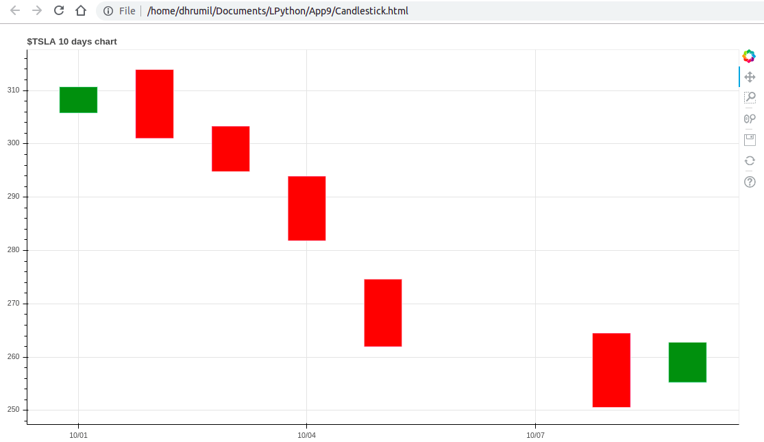
Building Candlestick Segments

We have a visually appealing chart and the body of the candle, but we are still left with the highs and lows. Just like all our lives, these candles too have highs and lows. Look at line 41 and you’ll know how to handle it, it’s that easy. What if it’s that simple in life too? We wish.

#Import libraries
from pandas_datareader import data
import datetime
from bokeh.plotting import figure, show, output_file

#Define time-frame
start_time = datetime.datetime(2018,10,1)
end_time = datetime.datetime(2018,10,9)

#Fetch the data
df = data.DataReader(name="TSLA",data_source="yahoo", start = start_time, end = end_time)

#Figure
chart = figure(x_axis_type="datetime", width = 1100, height = 600)
chart.title.text = "$TSLA 10 days chart"

#Body of candle
#Function 1 for Status
def inc_dec(c,o):
    if c > o:
        value = "Increase"
    elif o > c:
        value = "Decrease"
    else:
        value = "Equal"
    return value

df["Status"] = [inc_dec(c,o) for c, o in zip (df.Close,df.Open)]

#Function 2 and 3 for Middle Point and height
df["Middle"] = (df.Open + df.Close)/2
df["Height"] = abs(df.Close - df.Open)
print(df)

#hours to define width
hours = 12*60*60*1000

#Grid lines
chart.grid.grid_line_alpha = 0.3

#Segments
chart.segment(df.index, df.High, df.index, df.Low, color = "black")

#Creating actual body
chart.rect( df.index[df.Status=="Increase"],
            df.Middle[df.Status=="Increase"],
            hours,
            df.Height[df.Status=="Increase"],
            fill_color="green",
            line_color="white")

chart.rect( df.index[df.Status=="Decrease"],
            df.Middle[df.Status=="Decrease"],
            hours,
            df.Height[df.Status=="Decrease"],
            fill_color="red",
            line_color="white")

#Output file
output_file("Candlestick.html")
show(chart)

But hey, look, there we have it. A perfect candlestick chart for 10 days. How about we go long, for like 3 months or so? Wondering how it will look? Me too. Let’s feed our curiosity. The chart you see below is created using these 60 lines of code (I’ve added comments so it’s not even 60). Ain’t it amazing?

Endnotes

As we all know, we learn from visualizations far better than we learn from raw data. Building visualizations from data are really rewarding and with help of external libraries like Bokeh, Python’s visualization game is stronger than ever. In this post, you learned about stock market data, how to download it, what are candlestick charts and how to create them with help of Bokeh library.

*Originally published by Dhrumil Patel at *towardsdatascience.com

Learn More

☞ Learn Programming with Python Step by Step

☞ Complete Python: Go from zero to hero in Python

☞ An A-Z of useful Python tricks

☞ A Complete Machine Learning Project Walk-Through in Python

☞ Learning Python: From Zero to Hero

☞ MongoDB with Python Crash Course - Tutorial for Beginners

☞ Introduction to PyTorch and Machine Learning

☞ Python Tutorial for Beginners (2019) - Learn Python for Machine Learning and Web Development

☞ Complete Python Bootcamp: Go from zero to hero in Python 3

☞ Machine Learning A-Z™: Hands-On Python & R In Data Science

☞ Complete Python Masterclass

☞ Python and Django Full Stack Web Developer Bootcamp

☞ The Python Bible™ | Everything You Need to Program in Python

☞ The Python Mega Course: Build 10 Real World Applications

☞ Learning Python for Data Analysis and Visualization

#python #web-development