The majority of a data science project comprises of data cleaning and manipulation. Most of these data cleaning tasks can be broken down into six areas:
- Imputing Missing Values. Standard statistical constant imputing, KNN imputing.
- Outlier/Anomaly Detection. Isolation Forest, One Class SVM, Local Outlier Factor outlier detection algorithms.
- X-Variable Cleaning Methods. Applying custom functions, removing duplicates, replacing values.
- Y-Variable Cleaning Methods. Label encoding, dictionary mapping, one-hot encoding.
- Joining DataFrames. Concatenating, merging, and joining.
- Parsing Dates. Auto-format-detecting string-to-datetime converting, datetime objects to numbers.
Images created by author unless explicitly stated otherwise.
Imputing Missing Values
Missing values often plague data, and given that there are not too many of them, they can be imputed (filled in).
Simple Imputing Methods are statistical constant measures like the mean or the median which fills in NaN (missing values) with the statistical measure of each column. The parameter strategy can be substituted with ‘mean’, ‘median’, ‘most_frequent’ (mode), or ‘constant’ (a manual value with parameter fill_value).
from sklearn.impute import SimpleImputer
imputer = SimpleImputer(strategy='mean')
data = imputer.fit_transform(data)
KNN Imputing is the most popular and complex method for imputing missing values, in which the KNN algorithm finds other data points similar to one with a missing value within multidimensional space.
from sklearn.impute import KNNImputer
imputer = KNNImputer()
data = imputer.fit_transform(data)
Before using KNN and other distance-based algorithms, the data needs to be scaled or normalized to eliminate differences in scale (for example, one column representing number of children and another representing annual salary — these values cannot be taken at face value). Using KNN imputing follows the following process:
- Scale/normalize the data.
- KNN-impute to fill in missing values.
- Inverse scale/normalize the data.
Outlier/Anomaly Detection
Isolation Forest is an algorithm to return the anomaly score of a sample. The algorithm isolates observations by creating paths by randomly selecting a feature, randomly selecting a split value, the path length representing its normality. Shorter paths represent anomalies — when a forest of random trees collectively produce shorter path lengths for particular samples, they are highly likely to be anomalies.
from sklearn.ensemble import IsolationForest
identifier = IsolationForest().fit(X)
identifier.predict(X)
The output of predictions of the anomaly detector is an array of scores from -1 to 1, positive scores representing higher chances of being anomalies.
One Class SVM is another unsupervised method for detecting outliers, suited for high-dimensional distributions where an anomaly detection method like Isolation Forest would develop too much variance.
from sklearn.svm import OneClassSVM
identifier = OneClassSVM().fit(X)
identifier.predict(X)
Local Outlier Factor is the third of three commonly used outlier identifiers. The anomaly score of each sample — the Local Outlier Factor — measures the local deviation of density given a sample with respect to its neighbors. Based on the K-Nearest Neighbors, samples that have substantially lower density than their neighbors are considered outliers.
Because this algorithm is distance based, the data needs to be scaled or normalized before it is used. This algorithm can be seen as a non-linear high-variance alternative to Isolation Forest.
from sklearn.neighbors import LocalOutlierFactor
model = LocalOutlierFactor().fit(X)
model.predict(X)
For all three anomaly algorithms, it is the data scientist’s choice to eliminate all anomalies. Be sure that anomalies are not just data clusters themselves — make sure that the number of anomalies are not too excessive in number. A PCA visualization can confirm this.
X-Variable Cleaning Methods
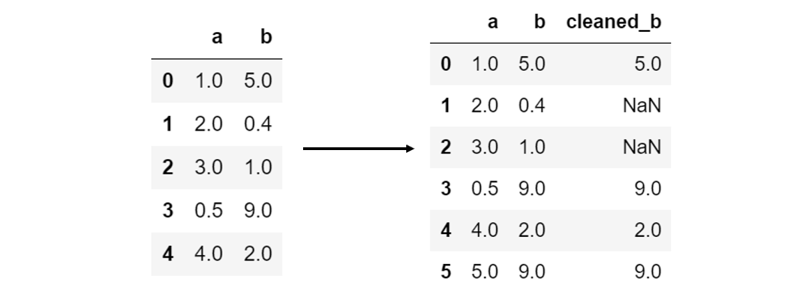
Applying a function to a column is often needed to clean it. In the case where cleaning cannot be done by a built-in function, you may need to write your own function or pass in an external built-in function. For example, say that all values of column b below 2 are invalid. A function to be applied can then act as a filter, returning NaN values for column elements that fail to pass the filter:
def filter_b(value):
     if value < 2:
          return np.nan
     else:
          return value
A new cleaned column, ‘cleaned_b’, can then be created by applying the filter using pandas’ .apply() function:
data['cleaned_b'] = data['b'].apply(filter_b)
Another common use case is converting data types. For instance, converting a string column into a numerical column could be done with data[‘target’].apply(float) using the Python built-in function float.
Removing duplicates is a common task in data cleaning. This can be done with data.drop_duplicates(), which removes rows that have the exact same values. Be cautious when using this — when the number of features is small, duplicate rows may not be errors in data collection. However, with large datasets and mostly continuous variables, the chance that duplicates are not errors is small.
Sampling data points is common when a dataset is too large (or for another purpose) and data points need to be randomly sampled. This can be done with data.sample(number_of_samples).
Renaming columns is done with .rename, where the parameter passed is a dictionary where the key is the original column name and the value is the renamed value. For example, data.rename({‘a’:1, ‘b’:3}) would rename the column ‘a’ to 1 and the column ‘b’ to 3.
Replacing values within the data can be done with data.replace(), which takes in two parameters to_replace and value, which represent values within the DataFrame that will be replaced by other values. This is helpful for the next section, imputing missing values, which can replace certain variables with np.nan so imputing algorithms can recognize them.
More handy pandas functions specifically for data manipulation can be found here:
7 Pandas Functions to Reduce Your Data Manipulation Stress
There’s a reason why Pandas have no gray hairs
Y-Variable Cleaning Methods
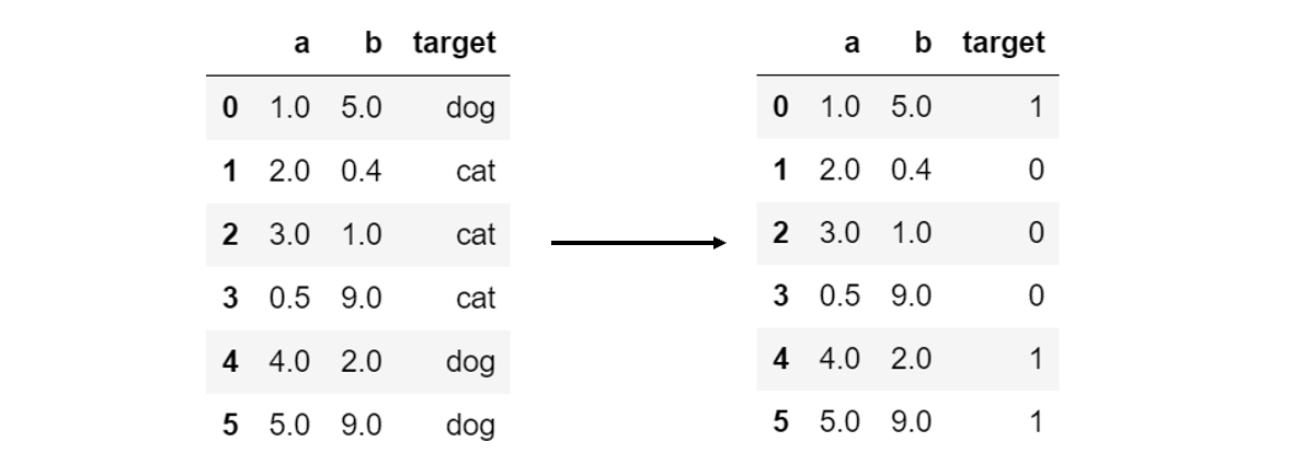
Label Encoding is required for categorical y-variables. For example, if data has two classes ‘cat’ and ‘dog’, they need to be mapped to 0 and 1, as machine learning algorithms operate purely on mathematical bases.
One simple way to do this is with the .map() function, which takes a dictionary in which keys are the original class names and the values are the elements they are to be replaced.
data['target'] = data['target'].map({'cat':0, 'dog':1})
However, in the case where there are too many classes to manually map with a dictionary, sklearn has an automated method:
from sklearn.preprocessing import LabelEncoder
encoder = LabelEncoder().fit(data['target'])
data['target'] = encoder.transform(data['target'])
The benefit of using this method of label encoding is that data can be inverse transformed — meaning from numerical values to their original classes — using encoder.inverse_transform(array).
One-Hot Encoding is advantageous over label encoding in certain scenarios with several classes when label encoding places quantitative measures on the data. Label encoding between classes ‘dog’, ‘cat’, and ‘fish’ to 0, 1, and 2 assumes that somehow ‘fish’ is larger than ‘dog’ or ‘dog’ is smaller than ‘cat’.
#data-science #data-analysis #ai #statistics #machine-learning #data analysis