Creating Bitcoin Trading Bots - Machine Learning
Creating Bitcoin trading bots don’t lose money. Let’s make cryptocurrency-trading agents using deep reinforcement learning
In this article we are going to create deep reinforcement learning agents that learn to make money trading Bitcoin. In this tutorial we will be using OpenAI’s gym and the PPO agent from the stable-baselines library, a fork of OpenAI’s baselines library.
The purpose of this series of articles is to experiment with state-of-the-art deep reinforcement learning technologies to see if we can create profitable Bitcoin trading bots. It seems to be the status quo to quickly shut down any attempts to create reinforcement learning algorithms, as it is “the wrong way to go about building a trading algorithm”. However, recent advances in the field have shown that RL agents are often capable of learning much more than supervised learning agents within the same problem domain. For this reason, I am writing these articles to see just how profitable we can make these trading agents, or if the status quo exists for a reason.
The Plan
- Create a gym environment for our agent to learn from
- Render a simple, yet elegant visualization of that environment
- Train our agent to learn a profitable trading strategy
Getting Started
For this tutorial, we are going to be using the Kaggle data set produced by Zielak. The .csv data file will also be available on my GitHub repo if you’d like to download the code to follow along. Okay, let’s get started.
First, let’s import all of the necessary libraries. Make sure to pip install any libraries you are missing.
import gym
import pandas as pd
import numpy as np
from gym import spaces
from sklearn import preprocessing
Next, let’s create our class for the environment. We’ll require a pandas data frame to be passed in, as well as an optional initial_balance, and a lookback_window_size, which will indicate how many time steps in the past the agent will observe at each step. We will default the commission per trade to 0.075%, which is Bitmex’s current rate, and default the serial parameter to false, meaning our data frame will be traversed in random slices by default.
We also call dropna() and reset_index() on the data frame to first remove any rows with NaN values, and then reset the frame’s index since we’ve removed data.
class BitcoinTradingEnv(gym.Env):
  """A Bitcoin trading environment for OpenAI gym"""
  metadata = {'render.modes': ['live', 'file', 'none']}
  scaler = preprocessing.MinMaxScaler()
  viewer = None

  def __init__(self, df, lookback_window_size=50,
                         commission=0.00075,
                         initial_balance=10000
                         serial=False):
    super(BitcoinTradingEnv, self).__init__()

  self.df = df.dropna().reset_index()
    self.lookback_window_size = lookback_window_size
    self.initial_balance = initial_balance
    self.commission = commission
    self.serial = serial

  # Actions of the format Buy 1/10, Sell 3/10, Hold, etc.
    self.action_space = spaces.MultiDiscrete([3, 10])

  # Observes the OHCLV values, net worth, and trade history
    self.observation_space = spaces.Box(low=0, high=1, shape=(10,
                    lookback_window_size + 1), dtype=np.float16)
Our action_space here is represented as a discrete set of 3 options (buy, sell, or hold) and another discrete set of 10 amounts (1/10, 2/10, 3/10, etc). When the buy action is selected, we will buy amount * self.balance worth of BTC. For the sell action, we will sell amount * self.btc_held worth of BTC. Of course, the hold action will ignore the amount and do nothing.
Our observation_space is defined as a continuous set of floats between 0 and 1, with the shape (10, lookback_window_size + 1). The + 1 is to account for the current time step. For each time step in the window, we will observe the OHCLV values, our net worth, the amount of BTC bought or sold, and the total amount in USD we’ve spent on or received from those BTC.
Next, we need to write our reset method to initialize the environment.
def reset(self):
  self.balance = self.initial_balance
  self.net_worth = self.initial_balance
  self.btc_held = 0

  self._reset_session()

  self.account_history = np.repeat([
    [self.net_worth],
    [0],
    [0],
    [0],
    [0]
		  ], self.lookback_window_size + 1, axis=1)

  self.trades = []

  return self._next_observation()
Here we use both self._reset_session and self._next_observation, which we haven’t defined yet. Let’s define them.
Trading Sessions

An important piece of our environment is the concept of a trading session. If we were to deploy this agent into the wild, we would likely never run it for more than a couple months at a time. For this reason, we are going to limit the amount of continuous frames in self.df that our agent will see in a row.
In our _reset_session method, we are going to first reset the current_step to 0. Next, we’ll set steps_left to a random number between 1 and MAX_TRADING_SESSION, which we will now define at the top of the file.
MAX_TRADING_SESSION = 100000 # ~2 months
Next, if we are traversing the frame serially, we will setup the entire frame to be traversed, otherwise we’ll set the frame_start to a random spot within self.df, and create a new data frame called active_df, which is just a slice of self.df from frame_start to frame_start + steps_left.
def _reset_session(self):
  self.current_step = 0

  if self.serial:
    self.steps_left = len(self.df) - self.lookback_window_size - 1
    self.frame_start = self.lookback_window_size
  else:
    self.steps_left = np.random.randint(1, MAX_TRADING_SESSION)
    self.frame_start = np.random.randint(
         self.lookback_window_size, len(self.df) - self.steps_left)

  self.active_df = self.df[self.frame_start -
       self.lookback_window_size:self.frame_start + self.steps_left]
One important side effect of traversing the data frame in random slices is our agent will have much more unique data to work with when trained for long periods of time. For example, if we only ever traversed the data frame in a serial fashion (i.e. in order from 0 to len(df)), then we would only ever have as many unique data points as are in our data frame. Our observation space could only even take on a discrete number of states at each time step.
However, by randomly traversing slices of the data frame, we essentially manufacture more unique data points by creating more interesting combinations of account balance, trades taken, and previously seen price action for each time step in our initial data set. Let me explain with an example.
At time step 10 after resetting a serial environment, our agent will always be at the same time within the data frame, and would have had3 choices to make at each time step: buy, sell, or hold. And for each of these 3 choices, another choice would then be required: 10%, 20%, …, or 100% of the amount possible. This means our agent could experience any of (1⁰³)¹⁰ total states, for a total of 1⁰³⁰ possible unique experiences.
Now consider our randomly sliced environment. At time step 10, our agent could be at any of len(df) time steps within the data frame. Given the same choices to make at each time step, this means this agent could experience any of len(df)³⁰ possible unique states within the same 10 time steps.
While this may add quite a bit of noise to large data sets, I believe it should allow the agent to learn more from our limited amount of data. We will still traverse our test data set in serial fashion, to get a more accurate understanding of the algorithm’s usefulness on fresh, seemingly “live” data.
Life Through The Agent’s Eyes
It can often be helpful to visual an environment’s observation space, in order to get an idea of the types of features your agent will be working with. For example, here is a visualization of our observation space rendered using OpenCV.
Each row in the image represents a row in our observation_space. The first 4 rows of frequency-like red lines represent the OHCL data, and the spurious orange and yellow dots directly below represent the volume. The fluctuating blue bar below that is the agent’s net worth, and the lighter blips below that represent the agent’s trades.
If you squint, you can just make out a candlestick graph, with volume bars below it and a strange morse-code like interface below that shows trade history. It looks like our agent should be able to learn sufficiently from the data in our observation_space, so let’s move on. Here we’ll define our _next_observation method, where we’ll scale the observed data from 0 to 1.
def _next_observation(self):
  end = self.current_step + self.lookback_window_size + 1

  obs = np.array([
    self.active_df['Open'].values[self.current_step:end],
    self.active_df['High'].values[self.current_step:end],
    self.active_df['Low'].values[self.current_step:end],
    self.active_df['Close'].values[self.current_step:end],
    self.active_df['Volume_(BTC)'].values[self.current_step:end],
  ])

  scaled_history = self.scaler.fit_transform(self.account_history)

  obs = np.append(obs, scaled_history[:, -(self.lookback_window_size
                                                     + 1):], axis=0)

  return obs
Taking Action
Now that we’ve set up our observation space, it’s time to write our step function, and in turn, take the agent’s prescribed action. Whenever self.steps_left == 0 for our current trading session, we will sell any BTC we are holding and call _reset_session(). Otherwise, we set the reward to our current net worth and only set done to True if we’ve run out of money.
def step(self, action):
  current_price = self._get_current_price() + 0.01
  self._take_action(action, current_price)
  self.steps_left -= 1
  self.current_step += 1

  if self.steps_left == 0:
    self.balance += self.btc_held * current_price
    self.btc_held = 0
    self._reset_session()

  obs = self._next_observation()
  reward = self.net_worth
  done = self.net_worth <= 0

  return obs, reward, done, {}
Taking an action is as simple as getting the current_price, determining the specified action, and either buying or selling the specified amount of BTC. Let’s quickly write _take_action so we can test our environment.
def _take_action(self, action, current_price):
  action_type = action[0]
  amount = action[1] / 10
  btc_bought = 0
  btc_sold = 0
  cost = 0
  sales = 0

  if action_type < 1:
    btc_bought = self.balance / current_price * amount
    cost = btc_bought * current_price * (1 + self.commission)
    self.btc_held += btc_bought
    self.balance -= cost

  elif action_type < 2:
    btc_sold = self.btc_held * amount
    sales = btc_sold * current_price  * (1 - self.commission)
    self.btc_held -= btc_sold
    self.balance += sales
Finally, in the same method, we will append the trade to self.trades and update our net worth and account history.
  if btc_sold > 0 or btc_bought > 0:
    self.trades.append({
      'step': self.frame_start+self.current_step,
      'amount': btc_sold if btc_sold > 0 else btc_bought,
      'total': sales if btc_sold > 0 else cost,
      'type': "sell" if btc_sold > 0 else "buy"
    })

  self.net_worth = self.balance + self.btc_held * current_price
  self.account_history = np.append(self.account_history, [
    [self.net_worth],
    [btc_bought],
    [cost],
    [btc_sold],
    [sales]
  ], axis=1)
Our agents can now initiate a new environment, step through that environment, and take actions that affect the environment. It’s time to watch them trade.
Watching Our Bots Trade
Our render method could be something as simple as calling print(self.net_worth), but that’s no fun. Instead we are going to plot a simple candlestick chart of the pricing data with volume bars and a separate plot for our net worth.
We are going to take the code in StockTradingGraph.py from the last article I wrote, and re-purposing it to render our Bitcoin environment. You can grab the code from my GitHub.
The first change we are going to make is to update self.df['Date'] everywhere to self.df['Timestamp'], and remove all calls to date2num as our dates already come in unix timestamp format. Next, in our render method we are going to update our date labels to print human-readable dates, instead of numbers.
from datetime import datetime
First, import the datetime library, then we’ll use the utcfromtimestamp method to get a UTC string from each timestamp and strftime to format the string in Y-m-d H:M format.
date_labels = np.array([datetime.utcfromtimestamp(x).strftime(
'%Y-%m-%d %H:%M') for x in self.df['Timestamp'].values[step_range]])
Finally, we change self.df['Volume'] to self.df['Volume_(BTC)'] to match our data set, and we’re good to go. Back in our BitcoinTradingEnv, we can now write our render method to display the graph.
def render(self, mode='human', **kwargs):
  if mode == 'human':
    if self.viewer == None:
      self.viewer = BitcoinTradingGraph(self.df,
                                        kwargs.get('title', None))

    self.viewer.render(self.frame_start + self.current_step,
                       self.net_worth,
                       self.trades,
                       window_size=self.lookback_window_size)
And voila! We can now watch our agents trade Bitcoin.
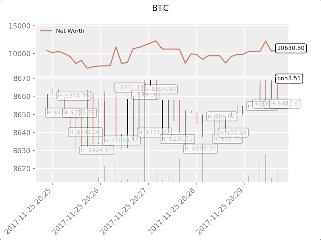
Matplotlib visualization of our agent trading Bitcoin
The green ghosted tags represent buys of BTC and the red ghosted tags represent sells. The white tag on the top right is the agent’s current net worth and the bottom right tag is the current price of Bitcoin. Simple, yet elegant. Now, it’s time to train our agent and see how much money we can make!
Training Time
One of the criticisms I received on my first article was the lack of cross-validation, or splitting the data into a training set and test set. The purpose of doing this is to test the accuracy of your final model on fresh data it has never seen before. While this was not a concern of that article, it definitely is here. Since we are using time series data, we don’t have many options when it comes to cross-validation.
For example, one common form of cross validation is called k-fold validation, in which you split the data into k equal groups and one by one single out a group as the test group and use the rest of the data as the training group. However time series data is highly time dependent, meaning later data is highly dependent on previous data. So k-fold won’t work, because our agent will learn from future data before having to trade it, an unfair advantage.
This same flaw applies to most other cross-validation strategies when applied to time series data. So we are left with simply taking a slice of the full data frame to use as the training set from the beginning of the frame up to some arbitrary index, and using the rest of the data as the test set.
slice_point = int(len(df) - 100000)
train_df = df[:slice_point]
test_df = df[slice_point:]
Next, since our environment is only set up to handle a single data frame, we will create two environments, one for the training data and one for the test data.
train_env = DummyVecEnv([lambda: BitcoinTradingEnv(train_df,
                         commission=0, serial=False)])
test_env = DummyVecEnv([lambda: BitcoinTradingEnv(test_df,
                        commission=0, serial=True)])
Now, training our model is as simple as creating an agent with our environment and calling model.learn.
model = PPO2(MlpPolicy,
             train_env,
             verbose=1,
             tensorboard_log="./tensorboard/")
model.learn(total_timesteps=50000)
Here, we are using tensorboard so we can easily visualize our tensorflow graph and view some quantitative metrics about our agents. For example, here is a graph of the discounted rewards of many agents over 200,000 time steps:
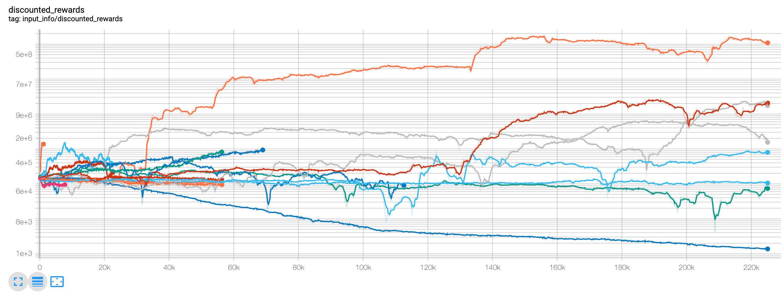
Wow, it looks like our agents are extremely profitable! Our best agent was even capable of 1000x’ing his balance over the course of 200,000 steps, and the rest averaged at least a 30x increase!
It was at this point that I realized there was a bug in the environment… Here is the new rewards graph, after fixing that bug:
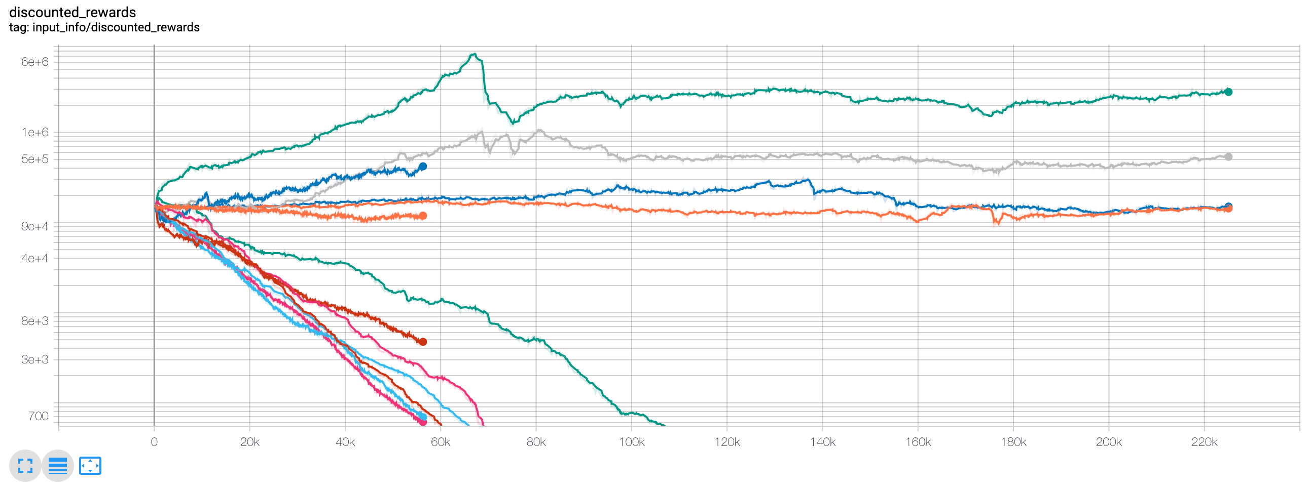
As you can see, a couple of our agents did well, and the rest traded themselves into bankruptcy. However, the agents that did well were able to 10x and even 60x their initial balance, at best. I must admit, all of the profitable agents were trained and tested in an environment without commissions, so it is still entirely unrealistic for our agent’s to make any real money. But we’re getting somewhere!
Let’s test our agents on the test environment (with fresh data they’ve never seen before), to see how well they’ve learned to trade Bitcoin.
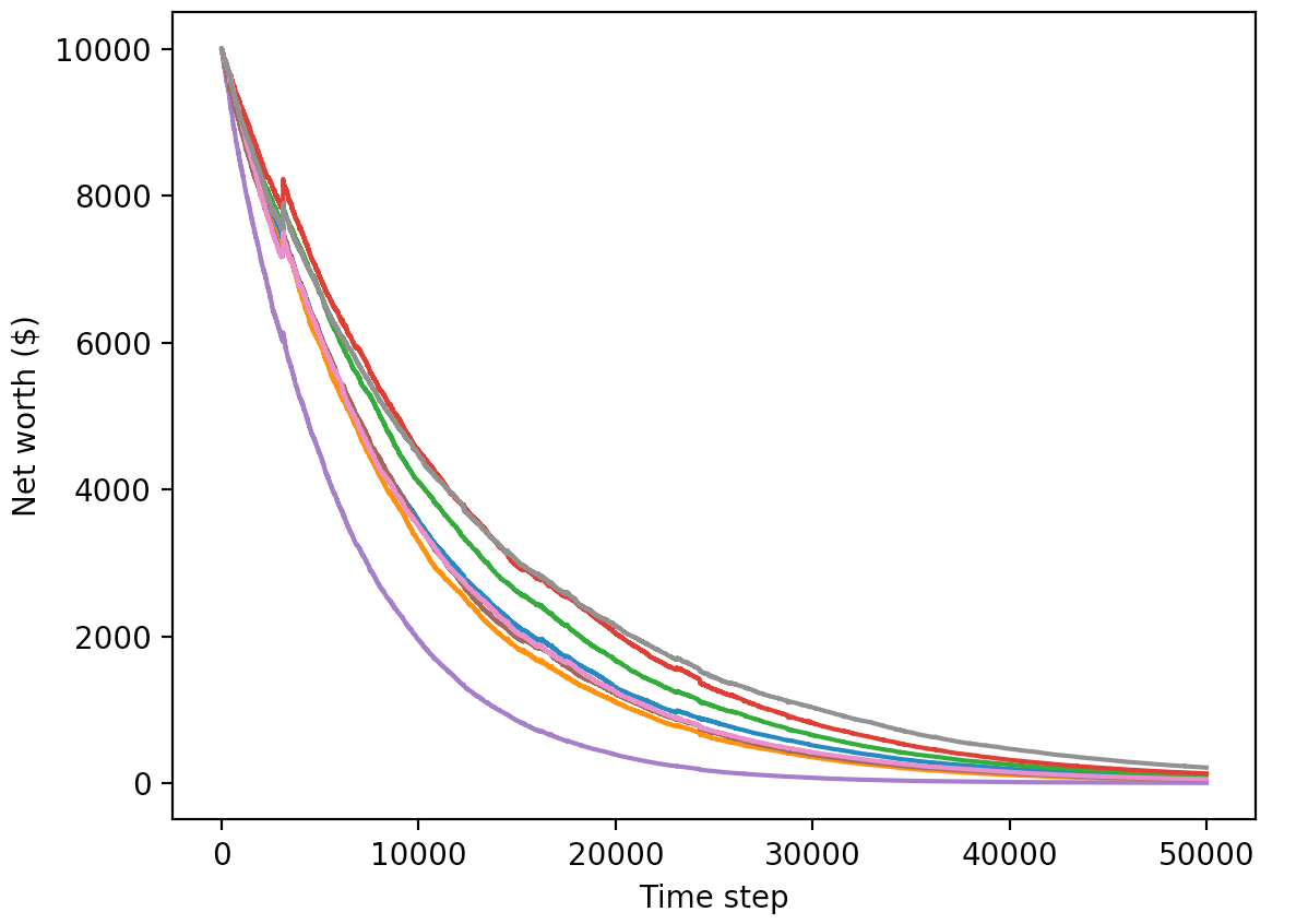
Our trained agents race to bankruptcy when trading on fresh, test data
Clearly, we’ve still got quite a bit of work to do. By simply switching our model to use stable-baseline’s A2C, instead of the current PPO2 agent, we can greatly improve our performance on this data set. Finally, we can update our reward function slightly, as per Sean O’Gorman’s advice, so that we reward increases in net worth, not just achieving a high net worth and staying there.
reward = self.net_worth - prev_net_worth
These two changes alone greatly improve the performance on the test data set, and as you can see below, we are finally able to achieve profitability on fresh data that wasn’t in the training set.
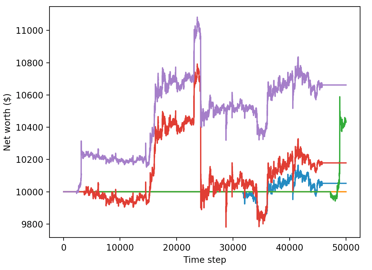
However, we can do much better. In order for us to improve these results, we are going to need to optimize our hyper-parameters and train our agents for much longer. Time to break out the GPU and get to work!
However, this article is already a bit long and we’ve still got quite a bit of detail to go over, so we are going to take a break here. In my next article, we will use Bayesian optimization to zone in on the best hyper-parameters for our problem space, and improve the agent’s model to achieve highly profitable trading strategies.
Conclusion
In this article, we set out to create a profitable Bitcoin trading agent from scratch, using deep reinforcement learning. We were able to accomplish the following:
- Created a Bitcoin trading environment from scratch using OpenAI’s gym.
- Built a visualization of that environment using Matplotlib.
- Trained and tested our agents using simple cross-validation.
- Tuned our agent slightly to achieve profitability.
While our trading agent isn’t quite as profitable as we’d hoped, it is definitely getting somewhere. Next time, we will improve on these algorithms through advanced feature engineering and Bayesian optimization to make sure our agents can consistently beat the market.
Thanks for reading! As always, all of the code for this tutorial can be found on _ GitHub. Leave a comment below if you have any questions or feedback,
#Python #Machine Learning #Deep Learning #Bitcoin #Trading