This post was written by Michael Nguyen, Machine Learning Research Engineer at AssemblyAI, and Niko Laskaris at Comet.ml. AssemblyAI uses Comet to log, visualize, and understand their model development pipeline.

Deep Learning has changed the game in speech recognition with the introduction of end-to-end models. These models take in audio, and directly output transcriptions. Two of the most popular end-to-end models today are Deep Speech by Baidu, and Listen Attend Spell (LAS) by Google. Both Deep Speech and LAS, are recurrent neural network (RNN) based architectures with different approaches to modeling speech recognition. Deep Speech uses the Connectionist Temporal Classification (CTC) loss function to predict the speech transcript. LAS uses a sequence to sequence network architecture for its predictions.

These models simplified speech recognition pipelines by taking advantage of the capacity of deep learning system to learn from large datasets. With enough data, you should, in theory, be able to build a super robust speech recognition model that can account for all the nuance in speech without having to spend a ton of time and effort hand engineering acoustic features or dealing with complex pipelines in more old-school GMM-HMM model architectures, for example.

Deep learning is a fast-moving field, and Deep Speech and LAS style architectures are already quickly becoming outdated. You can read about where the industry is moving in the Latest Advancement Section below.

How to Build Your Own End-to-End Speech Recognition Model in PyTorch

Let’s walk through how one would build their own end-to-end speech recognition model in PyTorch. The model we’ll build is inspired by Deep Speech 2 (Baidu’s second revision of their now-famous model) with some personal improvements to the architecture. The output of the model will be a probability matrix of characters, and we’ll use that probability matrix to decode the most likely characters spoken from the audio. You can find the full code and also run the it with GPU support on Google Colaboratory.

Preparing the data pipeline

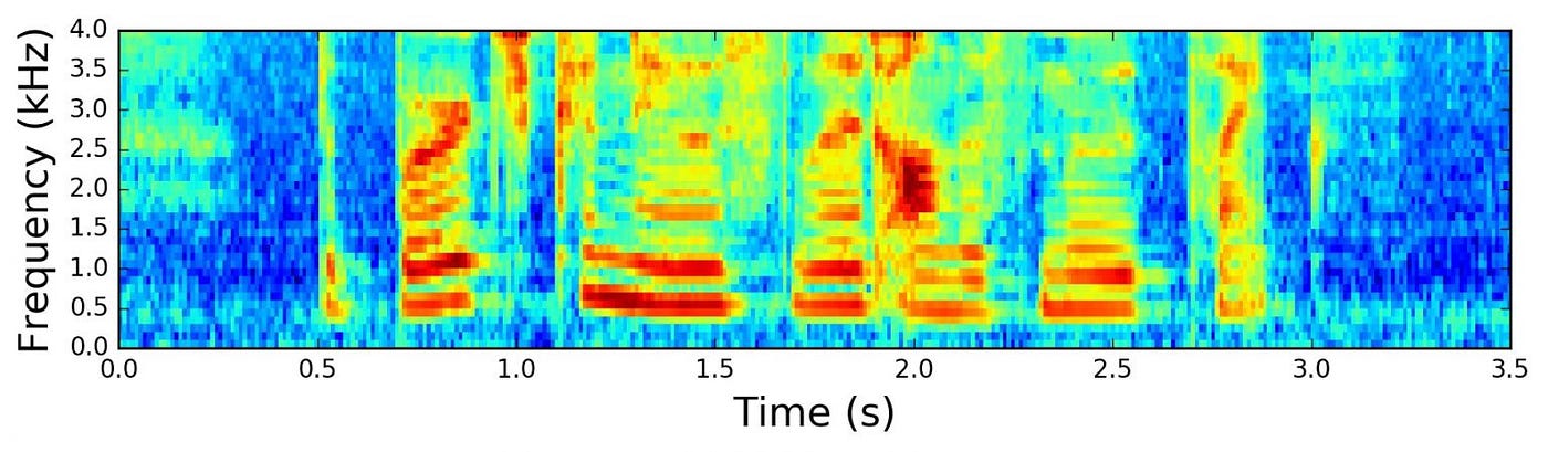
Data is one of the most important aspects of speech recognition. We’ll take raw audio waves and transform them into Mel Spectrograms.

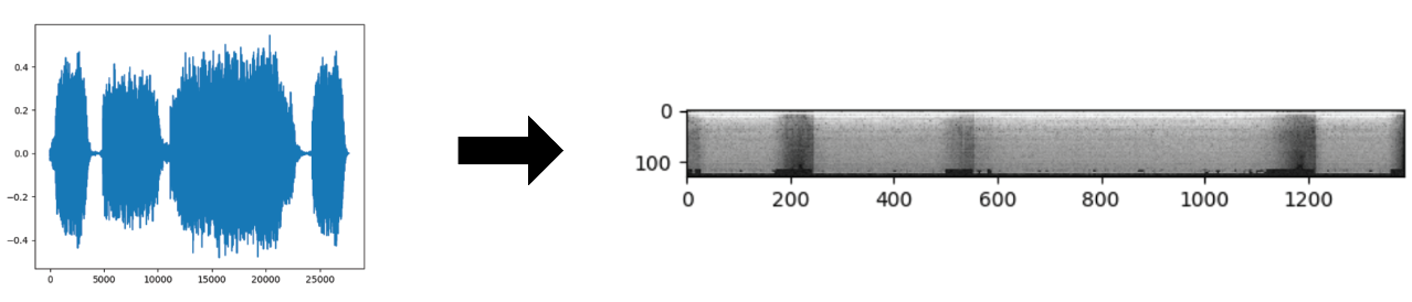
You can read more on the details about how that transformation looks from this excellent post here. For this post, you can just think of a Mel Spectrogram as essentially a picture of sound.

For handling the audio data, we are going to use an extremely useful utility called **torchaudio **which is a library built by the PyTorch team specifically for audio data. We’ll be training on a subset of LibriSpeech, which is a corpus of read English speech data derived from audiobooks, comprising 100 hours of transcribed audio data. You can easily download this dataset using torchaudio:

import torchaudio train_dataset = torchaudio.datasets.LIBRISPEECH("./", url="train-clean-100", download=True) 
test_dataset = torchaudio.datasets.LIBRISPEECH("./", url="test-clean", download=True)

Each sample of the dataset contains the waveform, sample rate of audio, the utterance/label, and more metadata on the sample. You can view what each sample looks like from the source code here.

Data Augmentation — SpecAugment

Data augmentation is a technique used to artificially increase the diversity of your dataset in order to increase your dataset size. This strategy is especially helpful when data is scarce or if your model is overfitting. For speech recognition, you can do the standard augmentation techniques, like changing the pitch, speed, injecting noise, and adding reverb to your audio data.

We found Spectrogram Augmentation (SpecAugment), to be a much simpler and more effective approach. SpecAugment, was first introduced in the paper SpecAugment: A Simple Data Augmentation Method for Automatic Speech Recognition, in which the authors found that simply cutting out random blocks of consecutive time and frequency dimensions improved the models generalization abilities significantly!

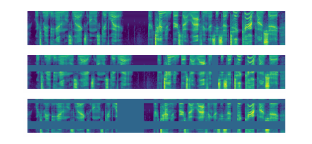
In PyTorch, you can use the** torchaudio** function FrequencyMasking to mask out the frequency dimension, and TimeMasking for the time dimension.

torchaudio.transforms.FrequencyMasking()
torchaudio.transforms.TimeMasking()

Now that we have the data, we’ll need to transform the audio into Mel Spectrograms, and map the character labels for each audio sample into integer labels:

class TextTransform:
    """Maps characters to integers and vice versa"""
    def __init__(self):
        char_map_str = """
        ' 0
        <SPACE> 1
        a 2
        b 3
        c 4
        d 5
        e 6
        f 7
        g 8
        h 9
        i 10
        j 11
        k 12
        l 13
        m 14
        n 15
        o 16
        p 17
        q 18
        r 19
        s 20
        t 21
        u 22
        v 23
        w 24
        x 25
        y 26
        z 27
        """
        self.char_map = {}
        self.index_map = {}
        for line in char_map_str.strip().split('\n'):
            ch, index = line.split()
            self.char_map[ch] = int(index)
            self.index_map[int(index)] = ch
        self.index_map[1] = ' '
def text_to_int(self, text):
        """ Use a character map and convert text to an integer sequence """
        int_sequence = []
        for c in text:
            if c == ' ':
                ch = self.char_map['']
            else:
                ch = self.char_map[c]
            int_sequence.append(ch)
        return int_sequence
def int_to_text(self, labels):
        """ Use a character map and convert integer labels to an text sequence """
        string = []
        for i in labels:
            string.append(self.index_map[i])
        return ''.join(string).replace('', ' ')
train_audio_transforms = nn.Sequential(
    torchaudio.transforms.MelSpectrogram(sample_rate=16000, n_mels=128),
    torchaudio.transforms.FrequencyMasking(freq_mask_param=15),
    torchaudio.transforms.TimeMasking(time_mask_param=35)
)
valid_audio_transforms = torchaudio.transforms.MelSpectrogram()
text_transform = TextTransform()
def data_processing(data, data_type="train"):
    spectrograms = []
    labels = []
    input_lengths = []
    label_lengths = []
    for (waveform, _, utterance, _, _, _) in data:
        if data_type == 'train':
            spec = train_audio_transforms(waveform).squeeze(0).transpose(0, 1)
        else:
            spec = valid_audio_transforms(waveform).squeeze(0).transpose(0, 1)
        spectrograms.append(spec)
        label = torch.Tensor(text_transform.text_to_int(utterance.lower()))
        labels.append(label)
        input_lengths.append(spec.shape[0]//2)
        label_lengths.append(len(label))
spectrograms = nn.utils.rnn.pad_sequence(spectrograms, batch_first=True).unsqueeze(1).transpose(2, 3)
    labels = nn.utils.rnn.pad_sequence(labels, batch_first=True)
return spectrograms, labels, input_lengths, label_lengths

Define the Model — Deep Speech 2 (but better)

Our model will be similar to the Deep Speech 2 architecture. The model will have two main neural network modules — N layers of Residual Convolutional Neural Networks (ResCNN) to learn the relevant audio features, and a set of Bidirectional Recurrent Neural Networks (BiRNN) to leverage the learned ResCNN audio features. The model is topped off with a fully connected layer used to classify characters per time step.

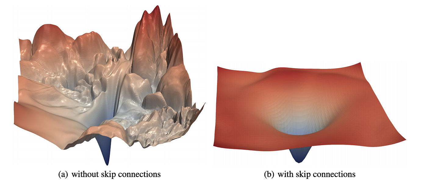
Convolutional Neural Networks (CNN) are great at extracting abstract features, and we’ll apply the same feature extraction power to audio spectrograms. Instead of just vanilla CNN layers, we choose to use Residual CNN layers. Residual connections (AKA skip connections) were first introduced in the paper Deep Residual Learning for Image Recognition, where the author found that you can build really deep networks with good accuracy gains if you add these connections to your CNN’s. Adding these Residual connections also helps the model learn faster and generalize better. The paper Visualizing the Loss Landscape of Neural Nets shows that networks with residual connections have a “flatter” loss surface, making it easier for models to navigate the loss landscape and find a lower and more generalizable minima.

Recurrent Neural Networks (RNN) are naturally great at sequence modeling problems. RNN’s processes the audio features step by step, making a prediction for each frame while using context from previous frames. We use BiRNN’s because we want the context of not only the frame before each step, but the frames after it as well. This can help the model make better predictions, as each frame in the audio will have more information before making a prediction. We use Gated Recurrent Unit (GRU’s) variant of RNN’s as it needs less computational resources than LSTM’s, and works just as well in some cases.

The model outputs a probability matrix for characters which we’ll use to feed into our decoder to extract what the model believes are the highest probability characters that were spoken.

#machine-learning #pytorch #assemblyai #deep learning