In this blog, I am going to discuss Graph Neural Network and its variants. Let us start with what graph neural networks are and what are the areas in which it can be applied. The sequence in which we proceed further is as follows:
Graph and its motivation
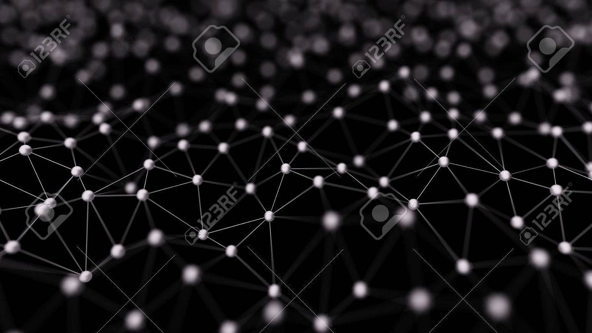
As the deep learning era has progressed so far, we have many states of the art solutions for datasets like text, images, videos etc. Mostly those algorithms consist of MLPs, RNNs, CNNs, Transformers, etc., which work outstandingly on the previously mentioned datasets. However, we may also come across some unstructured datasets like the ones shown below:
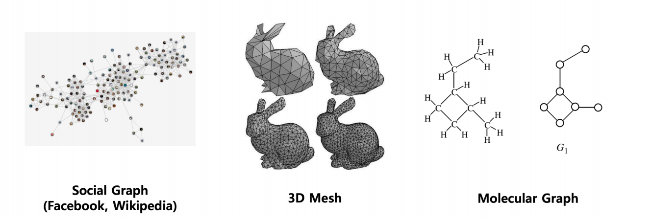
All you need to represent these systems are graphs and that is what we are going to discuss further.
Lets us briefly understand how a graph looks like:
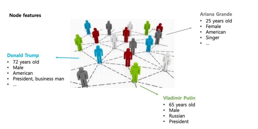
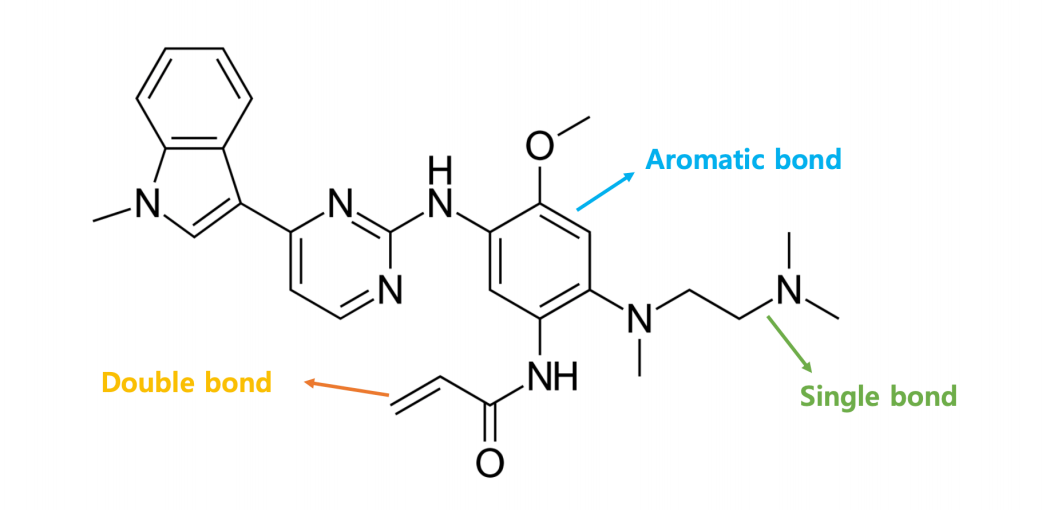
A graph G is represented by two key elements, {V, E} where V is the set of nodes and E is the set of edges defined among its nodes. A graph neural network has node features and edge features where node features represent the attributes of individual elements of a system and the edge features represent the relationship, interaction or connectivity amongst the elements of the system.
Node features:
Edge features:
A graph neural network can learn the inductive biases present in the system by not only producing the features of the elements of a system but understanding the interactions among them as well. The capability of learning of the inductive biases from a system makes it suitable for problems like few-shot learning, self-supervised or zero-shot learning.
We can use GNNs for purposes like node prediction, link prediction, finding embeddings for node, subgraph or graph etc. Now let us talk about graph convolutions.
Graph Convolutional Networks
So in a graph problem, we are given a graph G(V, E) and the goal is to learn the node and edge representations. For each vertex i, we need to have a feature vector**Vᵢ** and the relationship between nodes can be represented using an adjacency matrix A.
GCN can be represented using a simple neural network whose mathematical representation is as follows:
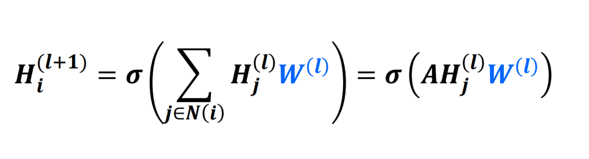
where **_Hᵢˡ _**is the feature vector of node i in the lᵗʰ layer, Wˡ is the weight matrix used for the _lᵗʰ _ layer and **_N(i) _**is the set of nodes in the neighbourhood of node i. Note that Hᵢ⁰=Vᵢ
Now as you can see the weights are shared for all the nodes in a given layer akin to conventional convolutional filters and the feature vector of a node is computed upon performing some mathematical operation(here weighted sum using the edge parameter) on its neighbourhood nodes(which also is similar to that of a CNN), we come up with the term Graph Convolutional Network and Wˡ can be called as a filter in layer _ l._
As it is evident, we see two issues here, the first being that while computing the feature vector for a node, we do not consider its own feature vector unless a self-loop is there. Secondly, the adjacency matrix used here is not a normalised one, so it can cause scaling problem or gradient explosion due to the large values of the edge parameters.
To solve the first issue a self-loop is enforced and to solve the second one, a normalized form of the adjacency matrix is used which is shown below:
Self-Loop: Â =A+I
Normalization: Â = (D^(-1/2))Â(D^(-1/2))
where I is an identity matrix of shape A and **D **is a diagonal matrix whose each diagonal value correspond to the degree of the respective node in matrix Â.
In each layer, the information is passed to a node from its neighbourhood, thus the process is called Message Passing.
Now let us talk about some variants of the simple graph convolution we talked about.
#data-science #deep-learning #machine-learning #graph-neural-networks #neural-networks