Tutorial explaining OO, NumPy, pandas, SQL and PySpark in Python
1. Introduction
A lot of companies are moving to cloud and consider what tooling shall be used for data analytics. On-premises, companies mostly use propriety software for advanced analytics, BI and reporting. However, this tooling may not be the most logical choice in a cloud environment. Reasons can be 1) lack of integration with cloud provider, 2) lack of big data support or 3) lack of support for new use cases such as machine learning and deep learning.
Python is a general-purpose programming language and is widely used for data analytics. Almost all cloud data platforms offer Python support and often new features become available in Python first. In this, Python can be seen as the Swiss Army knife of data analytics.
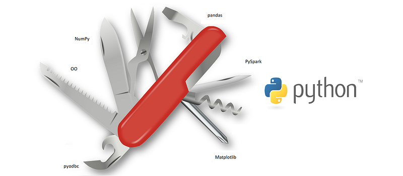
- Python as Swiss Army knife for data analytics
2. Objective
In this tutorial, two projects are created that take into account important features of Python. Projects are described as follows:
- In the first project, a Jupyter notebook is executed on a Data Science Virtual Machine (DSVM) in Azure. Object-oriented (OO) classes are created using inheritance, overloading and encapsulation of data. Subsequently, NumPy and pandas are used for data analytics. Finally, the data is stored in a database on the DSVM.
- In the second project, a Databricks notebook is executed on a Spark cluster with multiple VMs. PySpark is used to create a machine learning model.
Therefore, the following steps are executed:
-
- Prerequisites
-
- OO, NumPy, pandas and SQL with Jupyter on DSVM
-
- PySpark with Azure Databricks on Spark cluster
-
- Conclusion
It is a standalone tutorial in which the focus is to learn the different aspects of Python. The focus is less to “deep dive” in the separate aspects. In case you more interested in deep learning, see here or in devops for AI, refer to my previous blogs, here and with focus on security, see here.
3. Prerequisites
The following resources need to be created in the same resource group and in the same location.
- Data Science Virtual Machine (part 4)
- Azure Databricks Workspace (part 5)
4. OO, NumPy, pandas and sql with Jupyter on DSVM
In this part, a sample Python project with three classes. Using these classes, football player’s data is registered. The following steps are executed:
- 4a. Get started
- 4b. Object-oriented (OO) programming
- 4c. Matrix analytics using NumPy
- 4d. Statistical analytics using pandas
- 4e. Read/write to database
4a. Get started
Log in to your Windows Data Science Virtual Machine (DSVM). On the desktop, an overview of icons of preinstalled components can be found. Click on Jupyter short cut to start a Jupyter session.
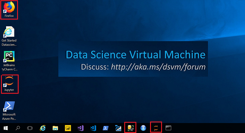
4a1. preinstalled components on DSVM needed in this tutorial
Subsequently, open the Jupyter command line session that can be found in the taskbar. Copy the URL and open this in a Firefox session.
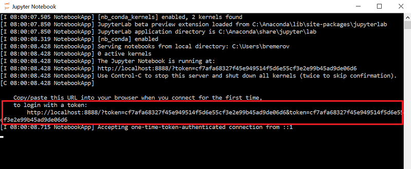
4a2. Localhost URL to be openen in Firefox
Then download the following notebook to the desktop of your DSVM:
https://raw.githubusercontent.com/rebremer/python_swiss_army_knife/master/SwissArmyKnifePython.ipynb
Finally, select to upload the notebook in your jupyter session. Then click on the run button in the menu to run code in a cell. The most important parts of the notebook are also discussed in the remaining of the chapter.
4b. Object-oriented (OO) programming
This part of the tutorial is inspired by the following tutorial by Theophano Mitsa. In this part, three classes are created to keep track of football players’ data. A snippet of the first class Player can be found below:
# Class 1: Player
class Player(object):
    _posList = {'goalkeeper', 'defender', 'midfielder', 'striker'}

    def __init__(self,name):
        self._playerName=name
        self._trainingList=[]
        self._rawData = np.empty((0,3), int)

    def setPosition(self, pos):
        if pos in self._posList:
            self._position=pos
            print(self._playerName + " is " + pos)
        else:
            raise ValueError("Value {} not in list.".format(pos))

    def setTraining(self, t, rawData):
        self._trainingList.append(t)
        self._rawData = np.append(self._rawData, rawData, axis=0)
    def getTrainingRawData(self):
        return self._rawData
    #def getTrainingFilter(self, stage, tt, date):
    # see github project for rest of code
The following can be seen in this class:
- A _rawData attribute is created when a new player is instantiated. This attribute is used to **encapsulate **training data with the setTraining method
- _rawData is created as **protected **variable. This tells a programmer that _rawData should be approached using get and set methods
Subsequently, class FirstTeamPlayer can be found below:
# Class 2: FirstTeamPlayer
class FirstTeamPlayer(Player):
    def __init__(self,ftp):
        Player.__init__(self, ftp)

    def setPosition(self,pos1, pos2):
        if pos1 in self._posList and pos2 in self._posList:
            self._posComp=pos1
            self._posCL=pos2
            print(self._playerName + " is " + pos1)
            print(self._playerName + " is " + pos2 + " in the CL")
        else:
            raise ValueError("Pos {},{} unknown".format(pos1, pos2))

    def setNumber(self,number):
        self._number=number
        print(self._playerName + " has number " + str(number))
The following can be seen in this class:
- FirstTeamPlayer **inherits **from Player class which means that all the attributes/methods of the Player class can also be used in FirstTeamPlayer
- Method setPosition is **overloaded **in FirstPlayerClass and has a new definition. Method setNumber is only available in FirstPlayerClass
Finally, a snippet of the training class can be found below:
# Class 3: Training
class Training(object):
    _stageList = {'ArenA', 'Toekomst', 'Pool', 'Gym'}
    _trainingTypeList = {'strength', 'technique', 'friendly game'}

    def __init__(self, stage, tt, date):
        if stage in self._stageList:
            self._stage = stage
        else:
            raise ValueError("Value {} not in list.".format(stage))
        if tt in self._trainingTypeList:
            self._trainingType = tt
        else:
            raise ValueError("Value {} not in list.".format(tt))

        #todo: Valid date test (no static type checking in Python)
        self._date = date

    def getStage(self):
        return self._stage

    def getTrainingType(self):
        return self._trainingType

    def getDate(self):
        return self._date
The following can be seen in this class:
- No static type checking is present in Python. For instance, a date attribute cannot be declared as date and an additional check has to be create
An example how the three classes are instantiated and are used can be found in the final snippet below:
# Construct two players, FirstTeamPlayer class inherits from Player
player1 = Player("Janssen")
player2 = FirstTeamPlayer("Tadic")
# SetPosition of player, method is overloaded in FirsTeamPlayer
player1.setPosition("goalkeeper")
player2.setPosition("midfielder", "striker")
# Create new traning object and add traningsdata to player object.
training1=Training('Toekomst', 'strength', date(2019,4,19))
player1.setTraining(training1, rawData=np.random.rand(1,3))
player2.setTraining(training1, rawData=np.random.rand(1,3))
# Add another object
training2=Training('ArenA', 'friendly game', date(2019,4,20))
player1.setTraining(training2, rawData=np.random.rand(1,3))
player2.setTraining(training2, rawData=np.random.rand(1,3))
4c. Matrix analytics using NumPy
NumPy is the fundamental package for scientific computing with Python. In this tutorial it will be used to do matrix analytics. Notice that attribute _rawData is already encapsulated in the Player class as a NumPy array. NumPy is often used with Matplotlib to visualize data. In the snippet below, the data is taken from player class and then some matrix operations are done, from basic to more advanced. Full example can be found in the github project.
# Take the matrix data from player objecs that were created earlier
m1=player1.getTrainingRawData()
m2=player2.getTrainingRawData()
# print some values
print(m1[0][1])
print(m1[:,0])
print(m1[1:3,1:3])
# arithmetic
tmp3=m1*m2 # [m2_11*m1_11,  ..,  m1_33*m2_33]
print(tmp3)
# matrix multiplication
tmp1 = m1.dot(m2) # [m1_11 * m2_11 + m1_23 * m2_32 +  m1_13 * m2_31,
                  #   ...,
                  # m1_31 * m2_13 + m1_23 * m2_32 +  m1_33 * m2_33]
print(tmp1)
# inverse matrix
m1_inv = np.linalg.inv(m1)
print("inverse matrix")
print(m1_inv)
print(m1.dot(m1_inv))
# singular value decomposition
u, s, vh = np.linalg.svd(m1, full_matrices=True)
print("singular value decomposition")
print(u)
print(s)
print(vh)
4d. Statistical analytics using pandas
Pandas is the package for high-performance, easy-to-use data structures and data analysis tools in Python. Under the hood, it also used NumPy for its array structure. In this tutorial it will be used to calculate some basic statistics. In the snippet below, the data is taken from player class and then some statistics operations are done. Full example can be found in the github project.
# Create the same matrices as earlier
m1=player1.getTrainingRawData()
m2=player2.getTrainingRawData()
# create column names to be added to pandas dataframe
columns = np.array(['col1', 'col2', 'col3'])

# Create pandas dataframe
df_1=pd.DataFrame(data=m1, columns=columns)
df_2=pd.DataFrame(data=m2, columns=columns)
# calculate basic statistics col1
print(df_1['col1'].sum())
print(df_1['col1'].mean())
print(df_1['col1'].median())
print(df_1['col1'].std())
print(df_1['col1'].describe())
# calculate correlation and covariance of dataframe
tmp1=df_1.cov()
tmp2=df_1.corr()

print("correlation:\n " + str(tmp1))
print("\n")
print("covariance:\n " + str(tmp2))
4e. Read/write to database
Finally, the data will be written to a SQL database. In this tutorial, the MSSQL database is used that is part of the DSVM. Look for the Microsoft SQL Server Management Studio (SSMS) icon that can be found in taskbar and start a new session. Log in using Windows Authentication, see also below.
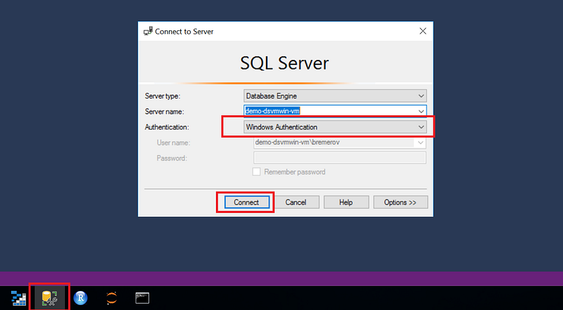
4e1. SSMS session using Windows Authentication
Look for “New Query” in the menu and start a new query session. Then
execute the following script:
USE [Master]
GO

CREATE DATABASE pythontest
GO

USE [pythontest]

CREATE TABLE [dbo].[trainingsdata]
(
 [col1] [float] NOT NULL,
 [col2] [float] NOT NULL,
 [col3] [float] NOT NULL
)
GO
Finally, the data can be written to and read from the database. Pandas dataframes will be used for this, see also the snippet below.
# import library
import pyodbc
# set connection variables
server  = '<<your vm name, which name of SQL server instance >>'
database = 'pythontest'
driver= '{ODBC Driver 17 for SQL Server}'
# Make connection to database
cnxn = pyodbc.connect('DRIVER='+driver+';SERVER='+server+';PORT=1433;DATABASE='+database + ';Trusted_Connection=yes;')
cursor = cnxn.cursor()
#Write results, use pandas dataframe
for index,row in df_1.iterrows():
    cursor.execute("INSERT INTO dbo.trainingsdata([col1],[col2],[col3]) VALUES (?,?,?)", row['col1'], row['col2'], row['col3'])
    cnxn.commit()
#Read results, use pandas dataframe
sql = "SELECT [col1], [col2], [col3] FROM dbo.trainingsdata"
df_1read = pd.read_sql(sql,cnxn)
print(df_1read)
cursor.close()
5. PySpark with Azure Databricks on Spark cluster
In the previous chapter, all code was run on a single machine. In case more data is generated or more advanced calculations need to be done (e.g. deep learning), the only possibility is to take a heavier machine an thus to scale upto execute the code. That is, compute cannot be distributed to other VMs.
Spark is an analytics framework that can distribute compute to other VMs and thus can **scale out **by adding more VMs to do work. This is most of times more efficient than having a “supercomputer” doing all the work. Python can be used in Spark and is often referred to as PySpark. In this tutorial, Azure Databricks will be used that is an Apache Spark-based analytics platform optimized for the Azure. In this, the following steps are executed.
- 5a. Get started
- 5b. Project setup
5a. Get started
Start your Azure Databricks workspace and go to Cluster. Create a new cluster with the following settings:
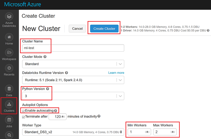
5a1. Create cluster
Subsequenly, select Workspace, right-click and then select import. In the radio button, select to import the following notebook using URL:
https://raw.githubusercontent.com/rebremer/devopsai_databricks/master/project/modelling/1_IncomeNotebookExploration.py
See also picture below:
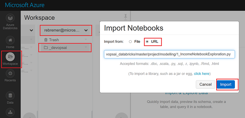
5a2. Import notebook
Select the notebook you imported in 4b and attach the notebook to the cluster you created in 4a. Make sure that the cluster is running and otherwise start it. Walk through the notebook cell by cell by using shortcut SHIFT+ENTER.
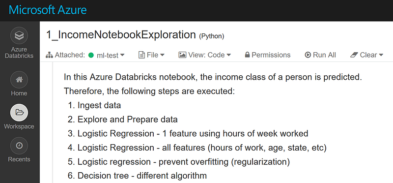
5a3. Run notebook
Finally, if you want to keep track of the model, create an HTTP endpoint of the model and/or create a DevOps pipeline of the project, see my advanced DevOps for AI tutorial here, and with focus on security, see here.
5b. Setup of project
In this project, a machine learning model is created that predicts the income class of a person using features as age, hours of week working, education. In this, the following steps are executed:
- Ingest, explore and prepare data as Spark Dataframe
- Logistic Regression — 1 feature using hours of week worked
- Logistic Regression — all features (hours of work, age, state, etc)
- Logistic regression — prevent overfitting (regularization)
- Decision tree — different algorithm, find the falgorithm performs best
Notice that pyspark.ml libraries are used to build the model. It is also possible to run scikit-learn libraries in Azure Databricks, however, then work would only be done be the driver (master) node and the compute is not distributed. See below a snippet of what pyspark packages are used.
from pyspark.ml import Pipeline, PipelineModel
from pyspark.ml.classification import LogisticRegression
from pyspark.ml.classification import DecisionTreeClassifier
#...
6. Conclusion
In this tutorial, two Python projects were created as follows:
- Jupyter notebook on a Data Science Virtual Machine using Object-oriented programming, NumPy, pandas for data analytics and SQL to store data
- Databricks notebook on a distributed Spark cluster with multiple VMs using PySpark to build a machine learning model
A lot of companies consider what tooling to use in the cloud for data analytics. In this, almost all cloud data analytics platforms have Python support and therefore, Python can be seen as the Swiss Army knife of data analytics. This tutorial may have helped you to explore the possibilites of Python.
#python #data-science
