Learn to group the data and summarize in several different ways, to use aggregate functions, data transformation, filter, map, apply a function in the DataFrame, and visualization using groupby.

Source: Unspalsh by Ilona Froehlich
Groupby is a very popular function in Pandas. This is very good at summarising, transforming, filtering, and a few other very essential data analysis tasks. In this article, I will explain the application of groupby function in detail with example.
Dataset
For this article, I will use a ‘Students Performance’ dataset from Kaggle. Please feel free download the dataset from here:
rashida048/Datasets
Contribute to rashida048/Datasets development by creating an account on GitHub.
Here I am importing the necessary packages and the dataset:
import pandas as pd
import numpy as np
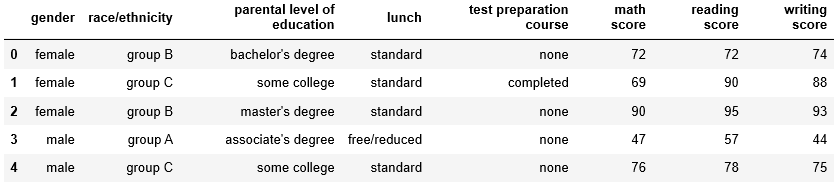
df = pd.read_csv('StudentsPerformance.csv')
df.head()
How Groupby Works?
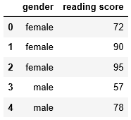
Groupby function splits the dataset based on criteria that you define. Here I am showing the process behind the groupby function. It will give you an idea, how much work we may have to do if we would not have groupby function. I will make a new smaller dataset of two columns only to demonstrate in this section. The columns are ‘gender’ and ‘reading score’.
test = df[['gender', 'reading score']]
test.head()
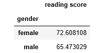
Let’s find out the average reading score gender-wise
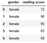
First, we need to split the dataset based on gender. Generate the data for females only.
female = test['gender'] == 'female'
test[female].head()
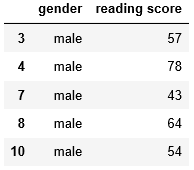
In the same way, generate the data for the males,
male = test['gender'] == 'male'
test[male].head()
Using females and males dataset above to calculate the mean reading score for females and males respectively.
fe_avg = test[female]['reading score'].mean()
male_avg = test[male]['reading score'].mean()
print(fe_avg, male_avg)
The mean reading score of females is 72.608 and the mean reading score for males is 65.473. Now, make a DataFrame for the mean reading score of females and males.
df_reading = pd.DataFrame({'Gender': ['female', 'male'], 'reading score': [fe_avg, male_avg]})
Now, let’s solve the same problem with the groupby function. Splitting the data based on gender and applying the ‘mean’ on it with just one simple line of code:
test.groupby('gender').mean()
This small piece of code gives the same result.
Groups in Groupby
I will use the original dataset ‘df’ now. Make groups of ‘race/ethnicity’.
race = df.groupby('race/ethnicity')
print(race)
Output: <pandas.core.groupby.generic.DataFrameGroupBy object at 0x0000023339DCE940>
It returns an object. Now check the datatype of ‘race’.
type(race)
Output: pandas.core.groupby.generic.DataFrameGroupBy
So, we generated a DataFrameGroupBy object. Calling groups on this DataFrameGroupBy object will return the indices of each group.
race.groups

#Here is the Output:
{'group A': Int64Index([  3,  13,  14,  25,  46,  61,  62,  72,  77,  82,  88, 112, 129,              143, 150, 151, 170, 228, 250, 296, 300, 305, 327, 356, 365, 368,              378, 379, 384, 395, 401, 402, 423, 428, 433, 442, 444, 464, 467,              468, 483, 489, 490, 506, 511, 539, 546, 571, 575, 576, 586, 589,              591, 597, 614, 623, 635, 651, 653, 688, 697, 702, 705, 731, 741,              769, 778, 805, 810, 811, 816, 820, 830, 832, 837, 851, 892, 902,              911, 936, 943, 960, 966, 972, 974, 983, 985, 988, 994],             dtype='int64'),  'group B': Int64Index([  0,   2,   5,   6,   7,   9,  12,  17,  21,  26,              ...              919, 923, 944, 946, 948, 969, 976, 980, 982, 991],             dtype='int64', length=190),  'group C': Int64Index([  1,   4,  10,  15,  16,  18,  19,  23,  27,  28,              ...              963, 967, 971, 975, 977, 979, 984, 986, 996, 997],             dtype='int64', length=319),  'group D': Int64Index([  8,  11,  20,  22,  24,  29,  30,  33,  36,  37,              ...              965, 970, 973, 978, 981, 989, 992, 993, 998, 999],             dtype='int64', length=262),  'group E': Int64Index([ 32,  34,  35,  44,  50,  51,  56,  60,  76,  79,              ...              937, 949, 950, 952, 955, 962, 968, 987, 990, 995],             dtype='int64', length=140)}
Have a look at the output above. Groupby function splits the data into subgroups and you can now see the indices of each subgroup. That’s great! But only the indices are not enough. We need to see the real data of each group. The function ‘get_group’ helps with that.
race.get_group('group B')

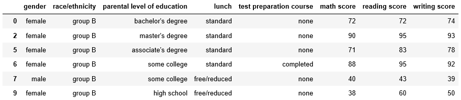
I am showing the part of the results here. The original output is much bigger.
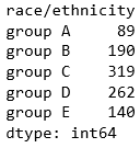
Find the size of each group
Calling size on the ‘race’ object will give the size of each group
race.size()
Loop over each group
You can loop over the groups. Here is an example:
for name, group in race:
    print(name, 'has', group.shape[0], 'data')

Grouping by multiple variables
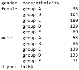
In all the examples above, we only grouped by one variable. But grouping by multiple variables is also possible. Here I am grouping by ‘race/ethnicity’ and ‘gender’. This should return the number of data of each race segregated by gender.
df.groupby(['gender', 'race/ethnicity']).size()
This example aggregates the data using ‘size’. There are other aggregate functions as well. Here is the list of all the aggregate functions:
sum()
mean()
size()
count()
std()
var()
sem()
min()
median()
Please try them out. Just replace any of these aggregate functions instead of the ‘size’ in the above example.
Using multiple aggregate functions
The way we can use groupby on multiple variables, using multiple aggregate functions is also possible. This next example will group by ‘race/ethnicity and will aggregate using ‘max’ and ‘min’ functions.
#data-science #pandas #data-analysis #towards-data-science #python #data analysis