Introduction
In the previous article we dived into the fundamental theory behind standard backpropagation and also introduced the different aspects that are responsible for practically optimizing the process. If you need a small recap or haven’t read it yet, you can check it out here. The third part of this blog series intends to introduce yet another essential concept known as learning rates and theoretically demonstrate how different implementations affect the convergence of a network.
Overview
1. Introduction to Learning Rates.
2. Deriving the Optimal learning rate in 1D — Taylor Method
3. Deriving the optimal learning rate in 1D — Graphical Method
4. Deriving the optimal learning rate in multidimension
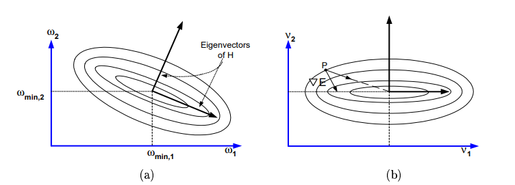
5. Introduction to Hessian Matrices
6. Eigenvectors and Eigenvalues
7. Revisiting input transformation
Please do note that all the images/diagrams in this article have been taken from the research paper and other sources as mentioned in the References below.
Introduction to Learning Rates
You must have come across this term a lot of times while referring different types of resources such as technical articles and other tutorials. Personally, I’ve always found that most of the time, this term is just briefly described and thrown into the mix without much explanation. However, as I happened to read more about it I realized that this concept was a lot more important than I thought it was.
So what do you mean by the ‘learning rate’ of a model?
The learning rate (also known as ‘step size’) is a positive hyper parameter that plays an important role in determining the amount by which a model adapts when the weights are updated. Hence, the value of the network’s learning rate needs to be carefully selected. If the value is too small, it will require more training epochs and the process will take more time whereas, if the value is too big, the network might converge very quickly and won’t be efficient.
This is where we introduce another term called optimal learning rate. Now this can be defined as the learning rate that can precisely move the weight to its minimum (most efficient) value in one step. The next few sections of this article will focus on how to derive the optimum learning rate in both one dimension and multiple dimensions.
But before we get on to the derivations, let’s see how different learning rates affect the efficiency of a model through the figures given below. (Here, _η and ηopt _represents the learning rate and optimal learning rate respectively)
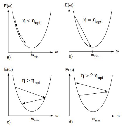
Gradient Descent for different learning rates ( Fig 6(i) in Source Paper)
The figure above illustrates 4 different cases which diagrammatically represents the graphical outcome of the relationship between the value of the learning rate and the optimal learning rate. These four cases can be categorized into the following.
Case 1: η < ηopt
The step size is small and the convergence requires multiple time steps.
Case 2: η = ηopt
This is the ideal case where the point of convergence is reached in a single step.
Case 3: η > ηopt
For the value of this learning rate, the weight will oscillate around Wmin and eventually converge.
Case 4: η > 2 ηopt
This is the worst case scenario which results in divergence. That is, the value of the weight will end up farther from Wmin than before.
Now that we’ve seen how learning rates can influence the process of convergence, let’s see how we can derive these values in different dimensions.
Deriving the optimal learning rate in one dimensional space
Method 1 — Taylor Series
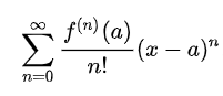
The Taylor series of a function is the infinite sum of terms that are expressed in terms of that function’s derivatives at a single point. It can be used to calculate the value of an entire function at every point, if the value of the function, and of all of its derivatives are known at a single point. The general formula for Taylor Series can be given by:
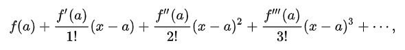
which can be generalized into,
Let’s apply this to the error function we have at hand. It’s best to get a pen and paper ready cause this might be a little hard to follow. Now in our case, the Taylor Series for the error function where the ‘single point’ is the current weight or Wc will be:

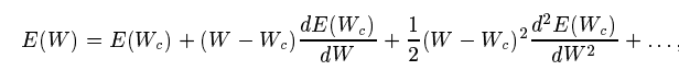
Eqn 21 in Source Paper
Differentiating both sides with respect to W, we get
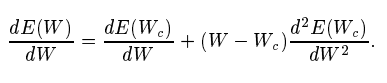
Eqn 22 in Source Paper
NOTE
If E is a quadratic function, the second order derivative is a constant and the higher order terms disappear after this step.
If we substitute W = Wmin and dE(Wmin)/dW = 0 and reframe the equation, we are left with
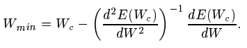
Eqn 23 in Source Paper
Comparing this equation with updation formula,
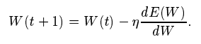
Eqn 11 in Source Paper
We finally get,

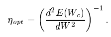
Eqn 24 in Source Paper
Method 2 — Graphical Method
If the last method seemed too confusing, another way to calculate this value is via the graphical representation of the error function we used before.
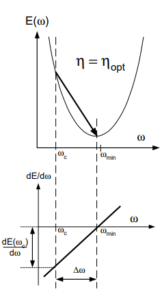
Fig 6(ii) in Source Paper
The given graph plots the gradient of E as a function of W. The gradient is a straight line since E is quadratic with a value of zero at the minimum and d(E(Wc))/dW at the current weight. The slope of this line is given by
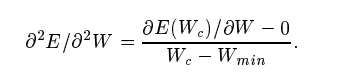
Eqn 25 in Source Paper
Solving this equation brings us back to the final few steps used in Method 1 after which we get the same value for the optimal learning rate.
#mathematics #machine-learning #deep-learning #research #gradient-descent #deep learning