Imagine that you are standing at the top of a mountain,blindfolded. You are asked to move the down the mountain and find the valley. What would you do? Since you are unsure of where and in which direction you need to move to reach the the ground, you would probably take little baby steps in some direction of the higher incline and try to figure out if that path leads to your destination. You would repeat this process until you reach the ground. This is exactly how Gradient Descent algorithm works.

Gradient Descent is an optimisation algorithm which is widely used in machine learning problems to minimise the cost function. So wait! what exactly is cost function?

Cost Function

Cost function is something which you want to minimise. For example, in case of linear regression, when you try to fit a line to your data-points, it may not fit exactly to each and every point in the data-set. Cost function helps us to measure how close the predicted values are to their corresponding real values. If x is the input variable and y is the output variable and h(hypothesis) is the predicted output of our learning algorithm.

hθ(x) = θ0 + θ1x , where θ0 is the intercept and θ1 is the gradient or slope.

Our aim here is to minimise the error between output y and the predicted output hθ(x). i.e. to minimise (hθ(x) — y)**2. This also called sum of the square error. Mathematically this cost function can be written as

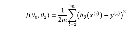
Cost function of Linear Regression

Our aim here is to determine values for θ which make the hypothesis as accurate as possible. In other words, minimise J(θ0,θ1) as much as possible.

So now that we have some idea about the cost function, let us try to understand how exactly Gradient Descent helps us to reduce this cost function.

Gradient Descent

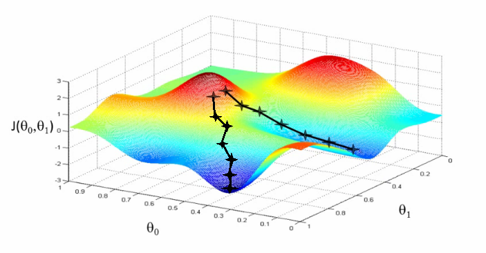
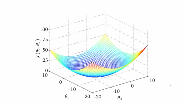
Gradient Descent (Image Source : Coursera)

We run our algorithm with some initial weights (θ0 and θ1) and gradient descent keeps updating these weights until it finds the optimal value for these weights which result in minimising the cost function.

In simple terms our aim to move from the red region to blue region as shown in the above picture. Initially we start at any random values of θ0 and θ1 (say 0,0). In every step we keep updating the values of θ0 and θ1 by small amount to try and reduce J(θ0,θ1). We need to keep updating these values until we reach a local minimum.

It is also interesting to see that there can be multiple local minima’s for a given problem as seen in the above picture. Our starting point determines which local minima we end up on.

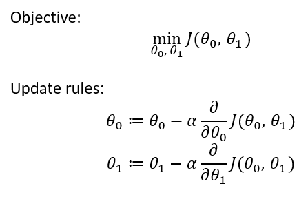
Gradient Descent Objective & Update rules

Here we take partial derivative of cost function with respect to each of the weights. Here **alpha **symbol indicates Learning Rate.

Learning Rate

It is important to set learning rate at an optimal level. If the learning rate is too high then it results in too big steps which in-turn results in overshooting the minima and the gradient descent never converges to local minima. If the learning rate is too low, steps will be very small and gradient descent will take a lot of time to converge to local minima.

Another important thing to note is that we don’t have to change the value of alpha in each step. Since as the gradient decent approaches the global minimum, the derivative term gets smaller, so even the update gets smaller and algorithm takes smaller steps as it approach the minimum.

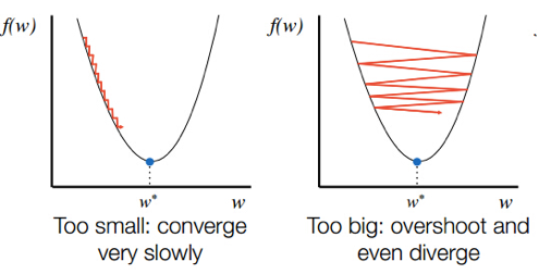
Learning Rate (Image source : GitHub)

In case of Linear Regression cost function is always a **convex function (bowl shaped) **and always has a single minimum. So gradient descent will always converge to global optima.

Cost function of Linear Regression

Conclusion

Gradient Descent helps us to reduce the cost function which results in increasing the accuracy of our machine learning model. Due to its ability to reduce error and since it can be applied to large data-sets with many variables, it is used in most of the machine learning algorithms.

#linear-regression #gradient-descent #machine-learning #cost-function #algorithms