A tour through history, how we ended up here, what capabilities we’ve unlocked, and where we go next?

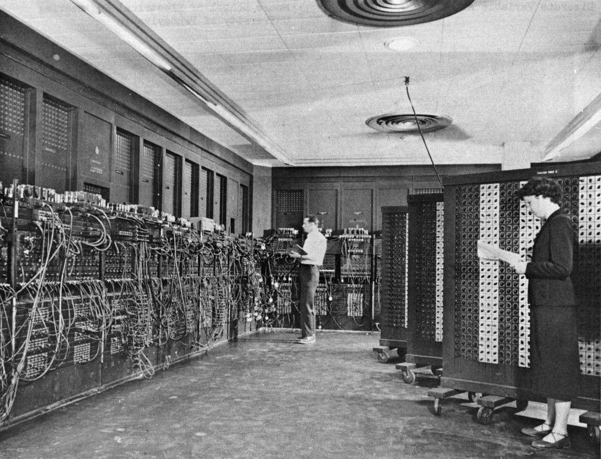
Glen Beck (background) and Betty Snyder (foreground) program ENIAC in BRL building 328. (U.S. Army photo, ca. 1947–1955) by U.S. Army Photo, n.d. Public Domain.

How It All Began (1940s)

A long time ago, in December 1945, the first electronic general-purpose digital computer was completed. It was called ENIAC (Electronic Numerical Integrator and Computer). It marked the start of an era where we produced computers for multiple classes of problems instead of custom building for each particular use case.

To compare the performance, ENIAC had a max clock of around 5 kHz on a single core, while the latest chip in an iPhone (Apple A13) has 2.66 GHz on 6 cores. This roughly translates to about four million times more cycles in a second, in addition to improvements in how much work can be accomplished in one of those cycles.

Historically, we’ve gone through cycles of expanding on the newest hardware advances to unlock new software engineering capabilities. There has been a pattern of increasing flexibility while also requiring more responsibility from the engineers. Inevitably there is a desire to reduce the additional burden that the engineers take while providing the same flexibility. This flexibility is enabled by implementing best practices that get teased out as we understand the patterns that work within a particular abstraction.

The Evolution of Data (1960s-1990s)

Historically servers were costly with limited storage, memory, and compute capabilities to solve the problems we wanted to solve without significant effort by the programmers such as memory management. In contrast, today, we now have languages with automated garbage collection to handle this for us. This is why C, C++, and FORTRAN were used so much and continue to be used for high-performance use cases where we try and drive as much efficiency and value out of a system as possible. Even today, most data analytics and Machine Learning frameworks in Python call out to C to ensure performance and only expose an API for the programmer.

To extract as much value as possible out of systems organizing data, companies like IBM invested heavily in particular models for storing, retrieving, and working with data. We have the hierarchical data model that was extremely prevalent during the days of big metal in the mainframe from this work. By creating a standard model, they reduced the amount of mental effort required to get a project started and increased knowledge that could be shared between projects.

An example hierarchical model for Pavement Improvement which breaks down into three categories, which might have their own categories. All structures must go downward and cannot connect back to a parent category. This forms a one-to-many relationship called a tree. “Hierarchical Model” by U.S. Department of Transportation, n.d. Public Domain.

Mainframes worked for the day’s problems but were prohibitively expensive, so only the largest enterprises such as banks were able to leverage them effectively. They were very efficient in traversing tree-like structures, but they imposed a very strict one-to-many relation that could be difficult to express for the programmer and make their applications hard to change.

Later on, the relational model was created, which powers most of our databases today. In the relational model, data is represented as sets of tuples (tables) with relations between them. A typical relationship is a foreign key which says that data in two tables should be related to each other. You can’t have a grade without a student to tie it to, and you can’t have a class without a teacher to teach the lesson.

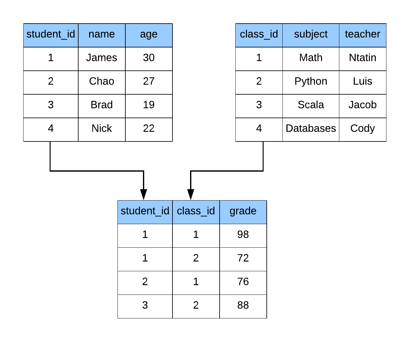
Relational diagram showing how tables are connected through ids.

Due to the structure that is applied to the data, we can define a standard language to interact with data in this form. The original inventor of the Relational Model also created its Structured Query Language (SQL), which is the de-facto standard for accessing data today. This is because SQL is easy to read, while also being extremely powerful. SQL is even Turing complete when the system has capabilities for recursion and windowing functions. Turing completeness roughly translates to the language can solve any computational problem given enough time. That’s an excellent theoretical property of SQL, but it doesn’t always mean it is the best tool for every job. This is why we use SQL to access and retrieve data, but leverage Python and other languages to do advanced analytics against the data.

Oracle released the first relational database product in 1979. These systems are called Relational Database Management Systems (RDBMS). Since then, dozens of commercial and open-source RDBMS have been released with various amounts of fanfare. These initial contributions to open source have led to Apache Software Foundation being the de-facto place for tooling in the “Big Data” space with its permissive license enabling commercial activities when leveraging the core source code of the libraries.

These systems work exceptionally well for managing and accessing data leveraging normalized data structures; however, as the data volumes grow, their performance starts to buckle under the stress of the load. We have several optimizations we can leverage to reduce the pressure on the systems, such as indexing, read-replicas, and more. The subject of optimizing RDBMS performance could be several more blog posts and books and is out of scope for this discussion.

The Connected World and All of Its Data (1990s)

Before computers were a staple in every home, and cell phones were in everyone’s pockets, there was significantly less communication and data surrounding that communication. Almost every website you go to has tracking enabled to understand the user experience better and provide personalized results back to their customers.

This explosion of data collection came from the ability to automate the collection where historically, users had to provide feedback in the form of surveys, phone calls, etc. Today we’re tracked by our activities, and our actions speak louder than our thoughts. Netflix no longer lets you rank or score movies, as they found that the signal wasn’t driving utilization of the ecosystem.

Google’s Search Index and the Need for MapReduce (early 2000s)

Google was one of the first companies to run into the scale of data collection that required sophisticated technology; however, in the late 90’s they didn’t have the enormous budget they have now as one of the most profitable companies in the world. Google’s competitive advantage is its data and how they leverage that data effectively. Let’s look into one of the earliest struggles they had as a business.

The engineering leads at Google had a hard problem to solve, and they could not afford the vastly more expensive enterprise-grade hardware on which traditional companies had relied. However, at the same time, they had the same if not more computing requirements than the other organizations did. Google had built a Frankenstein system to keep up with the growing demands of their business as well as the web in general. The parts in their servers were consumer-grade and were prone to failure, and the code that ran on top of them was not scalable or robust to these failure events either.

Jeff Dean and Sanjay Ghemawat were the engineering leadership at the time. They were diligently rewriting aspects of the Google codebase to be more resilient to failures. One of the biggest problems they had was that hardware would fail while jobs were running and needed to be restarted. As they kept solving for these problems within the code base, they noticed a consistent pattern was being followed, and they could instead abstract it and create a framework around it. This abstraction would come to be known as MapReduce.

MapReduce is a programming model defined in the two-step process, the map phase, and the reduce phase. Maps are applications of functions in an element-wise fashion, and reductions are aggregations. This framework provides a simple interface in which doing the work can be split in a smart way across different workers on a cluster. If we take some time to think through this without getting too deep, we realize that if we can split up our work, then we can also recover our work for a single failure without having to redo the entire set of work. Further, this translates into a much more scalable and robust system. There are many ways to improve the performance of a MapReduce system that we’ll go into as we evolve through the abstraction layers built-up from this concept over time.

“WordCountFlow”, by Magnai17, licensed under CC BY-SA 4.0.

By leveraging the MapReduce framework, Google effectively scaled up its infrastructure with commodity servers that were cheap and easy to build and maintain. They can address failures automatically in the code, and even further alert them that a server might need repairs or replacement parts. This effort saved them a significant amount of headaches as the web graph grew to be so large that no single computer yet alone supercomputer would handle the scale.

Both Jeff and Sanjay are still with Google and have collaborated on many technological advancements that shape the data landscape. A fantastic article was written about this inflection point for Google by James Somers at The New Yorker.

#spark #data #data-engineering #big-data #hadoop