In today’s video I will be showing you how the gradient descent algorithm works and how to code it in Python. Here is the definition of gradient descent from wikipedia for those who have no idea what it is:
“Gradient descent is a first-order iterative optimization algorithm for finding a local minimum of a differentiable function. To find a local minimum of a function using gradient descent, we take steps proportional to the negative of the gradient (or approximate gradient) of the function at the current point. But if we instead take steps proportional to the positive of the gradient, we approach a local maximum of that function; the procedure is then known as gradient ascent. Gradient descent was originally proposed by Cauchy in 1847.”

It is related to stochastic gradient descent and to mini-batch gradient descent, but it predates them. The main takeaway between all of these flavour of gradient descent is that the performance of the algorithm will change (speed and convergence) depending on how many point you are taking to calculate the gradient. If you take n=N it’s the original gradient descent, if you take n=1 it’s stochastic gradient descent if you take n=m where m is between 1 and N it’s mini-batch gradient descent.

Here is a very nice analogy of what gradient descent is doing, once again from wikipedia:

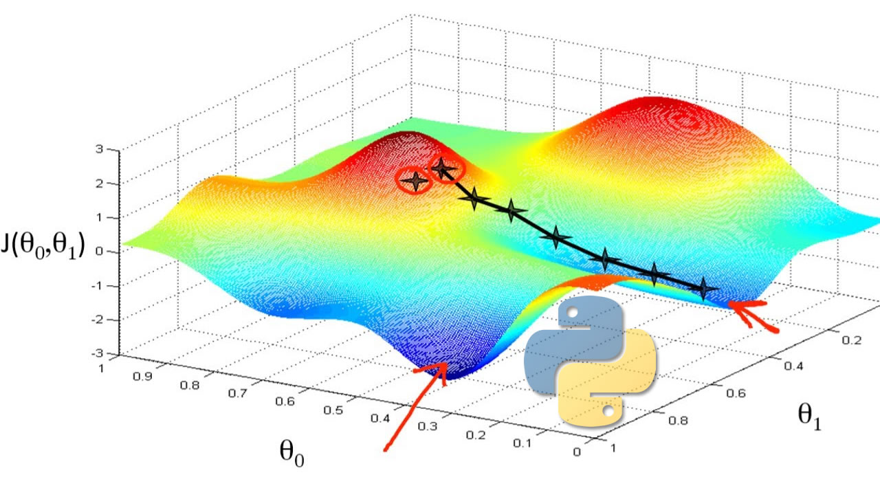
"The basic intuition behind gradient descent can be illustrated by a hypothetical scenario. A person is stuck in the mountains and is trying to get down (i.e. trying to find the global minimum). There is heavy fog such that visibility is extremely low. Therefore, the path down the mountain is not visible, so they must use local information to find the minimum. They can use the method of gradient descent, which involves looking at the steepness of the hill at their current position, then proceeding in the direction with the steepest descent (i.e. downhill). If they were trying to find the top of the mountain (i.e. the maximum), then they would proceed in the direction of steepest ascent (i.e. uphill). Using this method, they would eventually find their way down the mountain or possibly get stuck in some hole (i.e. local minimum or saddle point), like a mountain lake. However, assume also that the steepness of the hill is not immediately obvious with simple observation, but rather it requires a sophisticated instrument to measure, which the person happens to have at the moment. It takes quite some time to measure the steepness of the hill with the instrument, thus they should minimize their use of the instrument if they wanted to get down the mountain before sunset. The difficulty then is choosing the frequency at which they should measure the steepness of the hill so not to go off track.

In this analogy, the person represents the algorithm, and the path taken down the mountain represents the sequence of parameter settings that the algorithm will explore. The steepness of the hill represents the slope of the error surface at that point. The instrument used to measure steepness is differentiation (the slope of the error surface can be calculated by taking the derivative of the squared error function at that point). The direction they choose to travel in aligns with the gradient of the error surface at that point. The amount of time they travel before taking another measurement is the learning rate of the algorithm. See Backpropagation § Limitations for a discussion of the limitations of this type of “hill descending” algorithm. "

#python #machinelearning