Today, anything we can get data from can be measurable with the right knowledge and tools. WhatsApp is not the exception, thanks to the possibility that it offers us, to export complete conversations.

I want to introduce you to rwhatsapp, a small but very useful package, which provides what is necessary to work with WhatsApp text data in R as Data Frame.

Beginning. How do I export my conversations?

You can export every conversation in a very simple way, from your WhatsApp in any open conversation, from the options menu / More / Export chat. Immediately after this, you can send the complete history as a text file with the extension “.txt”.

The main function in the package is the rwa_read() function, which allows you to import TXT files directly, so you just need to provide the path to a file to load the messages directly as a Data Frame.

For this post, a friend very kindly (whom I thank for the trust) has shared her txt file of the chat with a person with whom she usually has a “casual relationship without commitments” for two years or more. For practical purposes we will analyze this conversation, visualizing some relevant data.

Export full chat from WhatsApp

Preparation and reading data

We will import some of the libraries that we will use, we will establish the text file that we will read, and to make this a little more interesting, we will segment by seasons of the year, from the summer of 2018 to the spring of 2020.

library(rwhatsapp)
library(lubridate)
library(tidyverse)
library(tidytext)
library(kableExtra)
library(RColorBrewer)
library(knitr)# LEEMOS EL CHAT A TRAVÉS DEL TXT EXPORTADO DESDE LA APP
miChat <- rwa_read(“miChat_1.txt”)# PREPARACIÓN DE DATOS PARA ANÁLISIS POR DATE/TIME
miChat <- miChat %>% 
 mutate(day = date(time)) %>% 
 mutate(
 # SEGMENTACIÓN POR MES
 estacion = case_when(
 day >= dmy(18082018) & day <= dmy(22092018) ~ “Verano 2018”,
 day >= dmy(23092018) & day <= dmy(20122018) ~ “Otoño 2018”,
 day >= dmy(21122018) & day <= dmy(20032019) ~ “Invierno 2018”,
 day >= dmy(21032019) & day <= dmy(21062019) ~ “Primavera 2019”,
 day >= dmy(22062019) & day <= dmy(23092019) ~ “Verano 2019”,
 day >= dmy(23092019) & day <= dmy(20122019) ~ “Otoño 2019”,
 day >= dmy(21122019) & day <= dmy(20032020) ~ “Invierno 2020”,
 day >= dmy(21032020) ~ “Primavera 2020”,
 T ~ “Fuera de rango”)
 ) %>% 
 mutate( estacion = factor(estacion) ) %>% 
 filter(!is.na(author))

Daily message frequency

Let’s look at the daily frequency of messages, assigning a personalized color palette for a first graph that shows the messages per day in a very visual way during the established seasons of the year.

# COLOR PALETTE
paleta.estaciones <- brewer.pal(8,"Set1")[c(7,5,1,3,4,2,6,8)]

# VERIFYING HOW MANY MESSAGES WERE SENT DURING THE PERIOD OF TIME
miChat %>% 
  group_by(estacion) %>% 
  count(day) %>%
  ggplot(aes(x = day, y = n, fill=estacion)) +
  geom_bar(stat = "identity") +
  scale_fill_manual(values=paleta.estaciones) +
  ylab("Número de mensajes") + xlab("Fecha") +
  ggtitle("Mensajes por día", "Frecuencia por estación del año") +
  theme_minimal() +
  theme( legend.title = element_blank(), 
         legend.position = "bottom")

We will obtain the following plot as a result. Something happened in Fall 2019, they stopped talking so often huh!

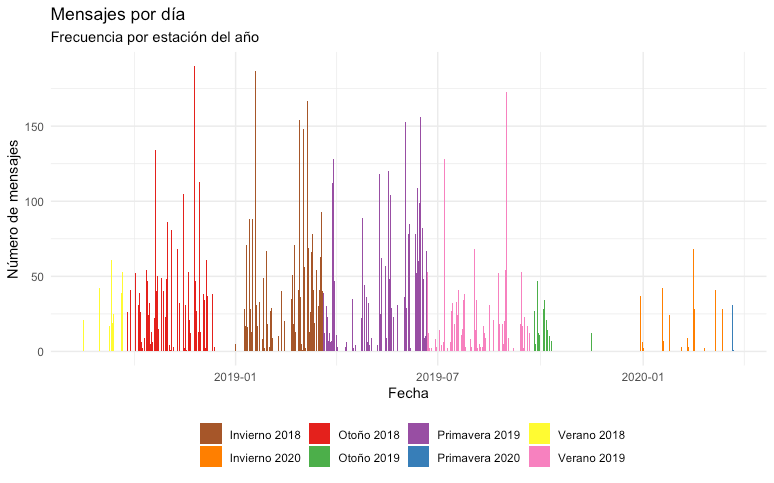
WhatsApp analysis with R — Frequency of daily messages

#data-analysis #data-visualization #dataviz #technology #rstudio #data analysis