For a recent hackathon that we did at STATWORX, some of our team members scraped minutely S&P 500 data from the Google Finance API. The data consisted of index as well as stock prices of the S&P’s 500 constituents. Having this data at hand, the idea of developing a deep learning model for predicting the S&P 500 index based on the 500 constituents prices one minute ago came immediately on my mind.

Playing around with the data and building the deep learning model with TensorFlow was fun and so I decided to write my first Medium.com story: a little TensorFlow tutorial on predicting S&P 500 stock prices. What you will read is not an in-depth tutorial, but more a high-level introduction to the important building blocks and concepts of TensorFlow models. The Python code I’ve created is not optimized for efficiency but understandability. The dataset I’ve used can be downloaded from here (40MB).

Note, that this story is a hands-on tutorial on TensorFlow. Actual prediction of stock prices is a really challenging and complex task that requires tremendous efforts, especially at higher frequencies, such as minutes used here.

Importing and preparing the data

Our team exported the scraped stock data from our scraping server as a csv file. The dataset contains n = 41266 minutes of data ranging from April to August 2017 on 500 stocks as well as the total S&P 500 index price. Index and stocks are arranged in wide format.

# Import data
data = pd.read_csv('data_stocks.csv')
# Drop date variable
data = data.drop(['DATE'], 1)
# Dimensions of dataset
n = data.shape[0]
p = data.shape[1]
# Make data a numpy array
data = data.values

The data was already cleaned and prepared, meaning missing stock and index prices were LOCF’ed (last observation carried forward), so that the file did not contain any missing values.

A quick look at the S&P time series using pyplot.plot(data['SP500']):

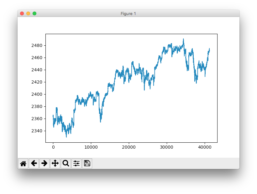
Time series plot of the S&P 500 index.

Note: This is actually the lead of the S&P 500 index, meaning, its value is shifted 1 minute into the future (this has already been done in the dataset). This operation is necessary since we want to predict the next minute of the index and not the current minute. Technically speaking, each row in the dataset contains the price of the S&P500 at t+1 and the constituent’s prices at T=t.

Preparing training and test data

The dataset was split into training and test data. The training data contained 80% of the total dataset. The data was not shuffled but sequentially sliced. The training data ranges from April to approx. end of July 2017, the test data ends end of August 2017.

# Training and test data
train_start = 0
train_end = int(np.floor(0.8*n))
test_start = train_end
test_end = n
data_train = data[np.arange(train_start, train_end), :]
data_test = data[np.arange(test_start, test_end), :]

There are a lot of different approaches to time series cross validation, such as rolling forecasts with and without refitting or more elaborate concepts such as time series bootstrap resampling. The latter involves repeated samples from the remainder of the seasonal decomposition of the time series in order to simulate samples that follow the same seasonal pattern as the original time series but are not exact copies of its values.

Data scaling

Most neural network architectures benefit from scaling the inputs (sometimes also the output). Why? Because most common activation functions of the network’s neurons such as tanh or sigmoid are defined on the [-1, 1] or [0, 1] interval respectively. Nowadays, rectified linear unit (ReLU) activations are commonly used activations which are unbounded on the axis of possible activation values. However, we will scale both the inputs and targets anyway. Scaling can be easily accomplished in Python using sklearn’s MinMaxScaler.

# Scale data
from sklearn.preprocessing import MinMaxScaler
scaler = MinMaxScaler()
data_train = scaler.fit_transform(data_train)
data_test = scaler.transform(data_test)
# Build X and y
X_train = data_train[:, 1:]
y_train = data_train[:, 0]
X_test = data_test[:, 1:]
y_test = data_test[:, 0]

Remark: Caution must be undertaken regarding what part of the data is scaled and when. A common mistake is to scale the whole dataset before training and test split are being applied. Why is this a mistake? Because scaling invokes the calculation of statistics e.g. the min/max of a variable. When performing time series forecasting in real life, you do not have information from future observations at the time of forecasting. Therefore, calculation of scaling statistics has to be conducted on training data and must then be applied to the test data. Otherwise, you use future information at the time of forecasting which commonly biases forecasting metrics in a positive direction.

Introduction to TensorFlow

TensorFlow is a great piece of software and currently the leading deep learning and neural network computation framework. It is based on a C++ low level backend but is usually controlled via Python (there is also a neat TensorFlow library for R, maintained by RStudio). TensorFlow operates on a graph representation of the underlying computational task. This approach allows the user to specify mathematical operations as elements in a graph of data, variables and operators. Since neural networks are actually graphs of data and mathematical operations, TensorFlow is just perfect for neural networks and deep learning. Check out this simple example (stolen from our deep learning introduction from our blog):

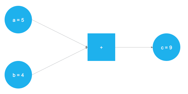
A very simple graph that adds two numbers together.

In the figure above, two numbers are supposed to be added. Those numbers are stored in two variables, a and b. The two values are flowing through the graph and arrive at the square node, where they are being added. The result of the addition is stored into another variable, c. Actually, a, b and c can be considered as placeholders. Any numbers that are fed into a and b get added and are stored into c. This is exactly how TensorFlow works. The user defines an abstract representation of the model (neural network) through placeholders and variables. Afterwards, the placeholders get “filled” with real data and the actual computations take place. The following code implements the toy example from above in TensorFlow:

# Import TensorFlow
import tensorflow as tf

# Define a and b as placeholders
a = tf.placeholder(dtype=tf.int8)
b = tf.placeholder(dtype=tf.int8)

# Define the addition
c = tf.add(a, b)

# Initialize the graph
graph = tf.Session()

# Run the graph
graph.run(c, feed_dict={a: 5, b: 4})

After having imported the TensorFlow library, two placeholders are defined using tf.placeholder(). They correspond to the two blue circles on the left of the image above. Afterwards, the mathematical addition is defined via tf.add(). The result of the computation is c = 9. With placeholders set up, the graph can be executed with any integer value for a and b. Of course, the former problem is just a toy example. The required graphs and computations in a neural network are much more complex.

Placeholders

As mentioned before, it all starts with placeholders. We need two placeholders in order to fit our model: X contains the network’s inputs (the stock prices of all S&P 500 constituents at time T = t) and Y the network’s outputs (the index value of the S&P 500 at time T = t + 1).

The shape of the placeholders correspond to [None, n_stocks] with [None] meaning that the inputs are a 2-dimensional matrix and the outputs are a 1-dimensional vector. It is crucial to understand which input and output dimensions the neural net needs in order to design it properly.

# Placeholder
X = tf.placeholder(dtype=tf.float32, shape=[None, n_stocks])
Y = tf.placeholder(dtype=tf.float32, shape=[None])

The None argument indicates that at this point we do not yet know the number of observations that flow through the neural net graph in each batch, so we keep if flexible. We will later define the variable batch_size that controls the number of observations per training batch.

Variables

Besides placeholders, variables are another cornerstone of the TensorFlow universe. While placeholders are used to store input and target data in the graph, variables are used as flexible containers within the graph that are allowed to change during graph execution. Weights and biases are represented as variables in order to adapt during training. Variables need to be initialized, prior to model training. We will get into that a litte later in more detail.

The model consists of four hidden layers. The first layer contains 1024 neurons, slightly more than double the size of the inputs. Subsequent hidden layers are always half the size of the previous layer, which means 512, 256 and finally 128 neurons. A reduction of the number of neurons for each subsequent layer compresses the information the network identifies in the previous layers. Of course, other network architectures and neuron configurations are possible but are out of scope for this introduction level article.

# Model architecture parameters
n_stocks = 500
n_neurons_1 = 1024
n_neurons_2 = 512
n_neurons_3 = 256
n_neurons_4 = 128
n_target = 1
# Layer 1: Variables for hidden weights and biases
W_hidden_1 = tf.Variable(weight_initializer([n_stocks, n_neurons_1]))
bias_hidden_1 = tf.Variable(bias_initializer([n_neurons_1]))
# Layer 2: Variables for hidden weights and biases
W_hidden_2 = tf.Variable(weight_initializer([n_neurons_1, n_neurons_2]))
bias_hidden_2 = tf.Variable(bias_initializer([n_neurons_2]))
# Layer 3: Variables for hidden weights and biases
W_hidden_3 = tf.Variable(weight_initializer([n_neurons_2, n_neurons_3]))
bias_hidden_3 = tf.Variable(bias_initializer([n_neurons_3]))
# Layer 4: Variables for hidden weights and biases
W_hidden_4 = tf.Variable(weight_initializer([n_neurons_3, n_neurons_4]))
bias_hidden_4 = tf.Variable(bias_initializer([n_neurons_4]))

# Output layer: Variables for output weights and biases
W_out = tf.Variable(weight_initializer([n_neurons_4, n_target]))
bias_out = tf.Variable(bias_initializer([n_target]))

It is important to understand the required variable dimensions between input, hidden and output layers. As a rule of thumb in multilayer perceptrons (MLPs, the type of networks used here), the second dimension of the previous layer is the first dimension in the current layer for weight matrices. This might sound complicated but is essentially just each layer passing its output as input to the next layer. The biases dimension equals the second dimension of the current layer’s weight matrix, which corresponds the number of neurons in this layer.

Designing the network architecture

After definition of the required weight and bias variables, the network topology, the architecture of the network, needs to be specified. Hereby, placeholders (data) and variables (weighs and biases) need to be combined into a system of sequential matrix multiplications.

Furthermore, the hidden layers of the network are transformed by activation functions. Activation functions are important elements of the network architecture since they introduce non-linearity to the system. There are dozens of possible activation functions out there, one of the most common is the rectified linear unit (ReLU) which will also be used in this model.

# Hidden layer
hidden_1 = tf.nn.relu(tf.add(tf.matmul(X, W_hidden_1), bias_hidden_1))
hidden_2 = tf.nn.relu(tf.add(tf.matmul(hidden_1, W_hidden_2), bias_hidden_2))
hidden_3 = tf.nn.relu(tf.add(tf.matmul(hidden_2, W_hidden_3), bias_hidden_3))
hidden_4 = tf.nn.relu(tf.add(tf.matmul(hidden_3, W_hidden_4), bias_hidden_4))

# Output layer (must be transposed)
out = tf.transpose(tf.add(tf.matmul(hidden_4, W_out), bias_out))

The image below illustrates the network architecture. The model consists of three major building blocks. The input layer, the hidden layers and the output layer. This architecture is called a feedforward network. Feedforward indicates that the batch of data solely flows from left to right. Other network architectures, such as recurrent neural networks, also allow data flowing “backwards” in the network.

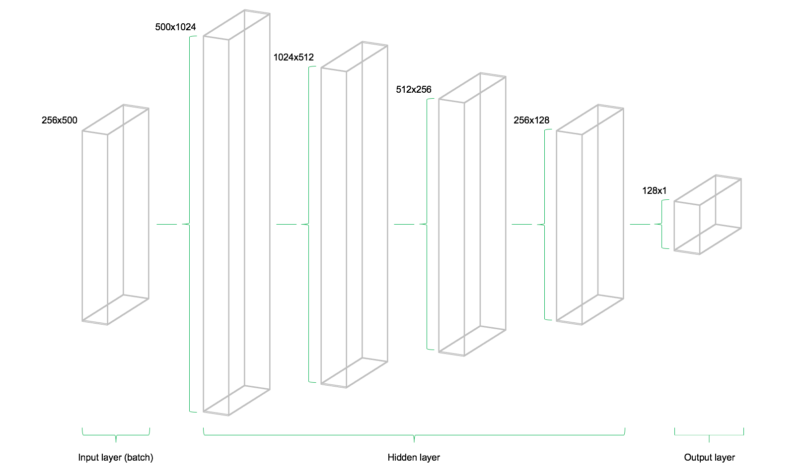
Cool technical illustration of our feedforward network architecture.

Cost function

The cost function of the network is used to generate a measure of deviation between the network’s predictions and the actual observed training targets. For regression problems, the mean squared error (MSE) function is commonly used. MSE computes the average squared deviation between predictions and targets. Basically, any differentiable function can be implemented in order to compute a deviation measure between predictions and targets.

# Cost function
mse = tf.reduce_mean(tf.squared_difference(out, Y))

However, the MSE exhibits certain properties that are advantageous for the general optimization problem to be solved.

Optimizer

The optimizer takes care of the necessary computations that are used to adapt the network’s weight and bias variables during training. Those computations invoke the calculation of so called gradients, that indicate the direction in which the weights and biases have to be changed during training in order to minimize the network’s cost function. The development of stable and speedy optimizers is a major field in neural network an deep learning research.

# Optimizer
opt = tf.train.AdamOptimizer().minimize(mse)

Here the Adam Optimizer is used, which is one of the current default optimizers in deep learning development. Adam stands for “Adaptive Moment Estimation” and can be considered as a combination between two other popular optimizers AdaGrad and RMSProp.

Initializers

Initializers are used to initialize the network’s variables before training. Since neural networks are trained using numerical optimization techniques, the starting point of the optimization problem is one the key factors to find good solutions to the underlying problem. There are different initializers available in TensorFlow, each with different initialization approaches. Here, I use the tf.variance_scaling_initializer(), which is one of the default initialization strategies.

# Initializers
sigma = 1
weight_initializer = tf.variance_scaling_initializer(mode="fan_avg", distribution="uniform", scale=sigma)
bias_initializer = tf.zeros_initializer()

Note, that with TensorFlow it is possible to define multiple initialization functions for different variables within the graph. However, in most cases, a unified initialization is sufficient.

Fitting the neural network

After having defined the placeholders, variables, initializers, cost functions and optimizers of the network, the model needs to be trained. Usually, this is done by minibatch training. During minibatch training random data samples of n = batch_size are drawn from the training data and fed into the network. The training dataset gets divided into n / batch_size batches that are sequentially fed into the network. At this point the placeholders X and Y come into play. They store the input and target data and present them to the network as inputs and targets.

A sampled data batch of X flows through the network until it reaches the output layer. There, TensorFlow compares the models predictions against the actual observed targets Y in the current batch. Afterwards, TensorFlow conducts an optimization step and updates the networks parameters, corresponding to the selected learning scheme. After having updated the weights and biases, the next batch is sampled and the process repeats itself. The procedure continues until all batches have been presented to the network. One full sweep over all batches is called an epoch.

The training of the network stops once the maximum number of epochs is reached or another stopping criterion defined by the user applies.

# Make Session
net = tf.Session()
# Run initializer
net.run(tf.global_variables_initializer())

# Setup interactive plot
plt.ion()
fig = plt.figure()
ax1 = fig.add_subplot(111)
line1, = ax1.plot(y_test)
line2, = ax1.plot(y_test*0.5)
plt.show()

# Number of epochs and batch size
epochs = 10
batch_size = 256

for e in range(epochs):

    # Shuffle training data
    shuffle_indices = np.random.permutation(np.arange(len(y_train)))
    X_train = X_train[shuffle_indices]
    y_train = y_train[shuffle_indices]

    # Minibatch training
    for i in range(0, len(y_train) // batch_size):
        start = i * batch_size
        batch_x = X_train[start:start + batch_size]
        batch_y = y_train[start:start + batch_size]
        # Run optimizer with batch
        net.run(opt, feed_dict={X: batch_x, Y: batch_y})

        # Show progress
        if np.mod(i, 5) == 0:
            # Prediction
            pred = net.run(out, feed_dict={X: X_test})
            line2.set_ydata(pred)
            plt.title('Epoch ' + str(e) + ', Batch ' + str(i))
            file_name = 'img/epoch_' + str(e) + '_batch_' + str(i) + '.jpg'
            plt.savefig(file_name)
            plt.pause(0.01)
# Print final MSE after Training
mse_final = net.run(mse, feed_dict={X: X_test, Y: y_test})
print(mse_final)

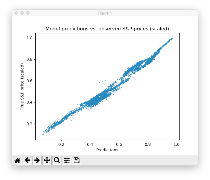
During the training, we evaluate the networks predictions on the test set — the data which is not learned, but set aside — for every 5th batch and visualize it. Additionally, the images are exported to disk and later combined into a video animation of the training process (see below). The model quickly learns the shape and location of the time series in the test data and is able to produce an accurate prediction after some epochs. Nice!

Video animation of the network’s test data prediction (orange) during training.

One can see that the networks rapidly adapts to the basic shape of the time series and continues to learn finer patterns of the data. This also corresponds to the Adam learning scheme that lowers the learning rate during model training in order not to overshoot the optimization minimum. After 10 epochs, we have a pretty close fit to the test data! The final test MSE equals 0.00078 (it is very low, because the target is scaled). The mean absolute percentage error of the forecast on the test set is equal to 5.31% which is pretty good. Note, that this is just a fit to the test data, no actual out of sample metrics in a real world scenario.

Please note that there are tons of ways of further improving this result: design of layers and neurons, choosing different initialization and activation schemes, introduction of dropout layers of neurons, early stopping and so on. Furthermore, different types of deep learning models, such as recurrent neural networks might achieve better performance on this task. However, this is not the scope of this introductory post.

Conclusion and outlook

The release of TensorFlow was a landmark event in deep learning research. Its flexibility and performance allows researchers to develop all kinds of sophisticated neural network architectures as well as other ML algorithms. However, flexibility comes at the cost of longer time-to-model cycles compared to higher level APIs such as Keras or MxNet. Nonetheless, I am sure that TensorFlow will make its way to the de-facto standard in neural network and deep learning development in research and practical applications. Many of our customers are already using TensorFlow or start developing projects that employ TensorFlow models. Also our data science consultants at STATWORX are heavily using TensorFlow for deep learning and neural net research and development. Let’s see what Google has planned for the future of TensorFlow. One thing that is missing, at least in my opinion, is a neat graphical user interface for designing and developing neural net architectures with TensorFlow backend. Maybe, this is something Google is already working on ;)

Update: I’ve added both the Python script as well as a (zipped) dataset to a Github repository. Feel free to clone and fork.

Final remarks

If you have any comments or questions on my story, feel free to comment below! I will try to answer them. Also, feel free to use my code or share this story with your peers on social platforms of your choice. Follow me on LinkedIn or Twitter, if you want to stay in touch.

Make sure, you also check the awesome STATWORX Blog for more interesting data science, ML and AI content straight from the our office in Frankfurt, Germany!

If you’re interested in more quality content like this, join my mailing list, constantly bringing you new data science, machine learning and AI reads and treats from me and my team right into your inbox!

#TensorFlow #ai #programming