Traditional ASR (Signal Analysis, MFCC, DTW, HMM & Language Modelling) and DNNs (Custom Models & Baidu DeepSpeech Model) on Indian Accent Speech
Courtesy_: _Speech and Music Technology Lab, IIT Madras

Notwithstanding an approved Indian-English accent speech, accent-less enunciation is a myth. Irregardless of the racial stereotypes, our speech is naturally shaped by the vernacular we speak, and the Indian vernaculars are numerous! Then how does a computer decipher speech from different Indian states, which even Indians from other states, find ambiguous to understand?
**ASR (Automatic Speech Recognition) **takes any continuous audio speech and output the equivalent text . In this blog, we will explore some challenges in speech recognition with focus on the speaker-independent recognition, both in theory and practice.
The** challenges in ASR** include
- Variability of volume
- Variability of words speed
- Variability of Speaker
- Variability of** pitch**
- Word boundaries: we speak words without pause.
- **Noises **like background sound, audience talks etc.
Lets address** each of the above problems** in the sections discussed below.
The complete source code of the above studies can be found here.
Models in speech recognition can conceptually be divided into:
- Acoustic model: Turn sound signals into some kind of phonetic representation.
- Language model: houses domain knowledge of words, grammar, and sentence structure for the language.
Signal Analysis
When we speak we create sinusoidal vibrations in the air. Higher pitches vibrate faster with a higher frequency than lower pitches. A microphone transduce acoustical energy in vibrations to electrical energy.

If we say “Hello World’ then the corresponding signal would contain 2 blobs

Some of the vibrations in the signal have higher amplitude. The amplitude tells us how much acoustical energy is there in the sound
Our speech is made up of many frequencies at the same time, i.e. it is a sum of all those frequencies. To analyze the signal, we use the component frequencies as features. **Fourier transform **is used to break the signal into these components.

We can use this splitting technique to convert the sound to a Spectrogram, where **frequency **on the vertical axis is plotted against time. The intensity of shading indicates the amplitude of the signal.

Spectrogram of the hello world phrase
To create a Spectrogram,
- **Divide the signal **into time frames.
- Split each frame signal into frequency components with an FFT.
- Each time frame is now represented with a** vector of amplitudes** at each frequency.

one dimensional vector for one time frame
If we line up the vectors again in their time series order, we can have a visual picture of the sound components, the Spectrogram.

Spectrogram can be lined up with the original audio signal in time
Next, we’ll look at Feature Extraction techniques which would reduce the noise and dimensionality of our data.

Unnecessary information is encoded in Spectrograph
Feature Extraction with MFCC
Mel Frequency Cepstrum Coefficient Analysis is the reduction of an audio signal to essential speech component features using both Mel frequency analysis and Cepstral analysis. The range of frequencies are reduced and binned into groups of frequencies that humans can distinguish. The signal is further separated into source and filter so that variations between speakers unrelated to articulation can be filtered away.
a) Mel Frequency Analysis
Only **those frequencies humans can hear are **important for recognizing speech. We can split the frequencies of the Spectrogram into bins relevant to our own ears and filter out sound that we can’t hear.
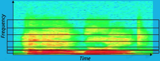
Frequencies above the black line will be filtered out
b) Cepstral Analysis
We also need to separate the elements of sound that are speaker-independent. We can think of a human voice production model as a combination of source and filter, where the source is unique to an individual and the filter is the articulation of words that we all use when speaking.

Cepstral analysis relies on this model for separating the two. The cepstrum can be extracted from a signal with an algorithm. Thus, we drop the component of speech unique to individual vocal chords and preserving the shape of the sound made by the vocal tract.
Cepstral analysis combined with Mel frequency analysis get you 12 or 13 MFCC features related to speech. **Delta and Delta-Delta MFCC features **can optionally be appended to the feature set, effectively doubling (or tripling) the number of features, up to 39 features, but gives better results in ASR.

Thus MFCC (Mel-frequency cepstral coefficients) Features Extraction,
- Reduced the dimensionality of our data and
- We squeeze noise out of the system
So there are 2 Acoustic Features for Speech Recognition:
- Spectrograms
- Mel-Frequency Cepstral Coefficients (MFCCs):
When you construct your pipeline, you will be able to choose to use either spectrogram or MFCC features. Next, we’ll look at sound from a language perspective, i.e. the phonetics of the words we hear.
Phonetics
Phonetics is the study of sound in human speech. Linguistic analysis is used to break down human words into their smallest sound segments.

phonemes define the distinct sounds
- Phoneme is the smallest sound segment that can be used to distinguish one word from another.
- Grapheme, in contrast, is the smallest distinct unit written in a language. Eg: English has 26 alphabets plus a space (27 graphemes).
Unfortunately, we can’t map phonemes to grapheme, as some letters map to multiple phonemes & some phonemes map to many letters. For example, the C letter sounds different in cat, chat, and circle.

Phonemes are often a useful intermediary between speech and text. If we can successfully produce an acoustic model that decodes a sound signal into phonemes the remaining task would be to map those phonemes to their matching words. This step is called Lexical Decoding, named so as it is based on a lexicon or dictionary of the data set.

If we want to train a limited vocabulary of words we might just skip the phonemes. If we have a large vocabulary, then converting to smaller units first, reduces the total number of comparisons needed.
Acoustic Models and the Trouble with Time
With feature extraction, we’ve addressed noise problems as well as variability of speakers. But we still haven’t solved the problem of matching variable lengths of the same word.
Dynamic Time Warping (DTW) calculates the similarity between two signals, even if their time lengths differ. This can be used to align the sequence data of a new word to its most similar counterpart in a dictionary of word examples.

2 signals mapped with Dynamic Time Warping
#deep-speech #speech #deep-learning #speech-recognition #machine-learning #deep learning