Introduction:

In this article, I will be explaining how to use the concept of regression, in specific logistic regression to the problems involving classification. Classification problems are everywhere around us, the classic ones would include mail classification, weather classification, etc. All these data, if needed can be used to train a Logistic regression model to predict the class of any future example.

Context:

This article is going to cover the following sub-topics:

1. Introduction to classification problems.
2. Logistic regression and all its properties such as hypothesis, decision boundary, cost, cost function, gradient descent, and its necessary analysis.
3. Developing a logistic regression model from scratch using python, pandas, matplotlib, and seaborn and training it on the Breast cancer dataset.
4. Training an in-built Logistic regression model from sklearn using the Breast cancer dataset to verify the previous model.

Introduction to classification problems:

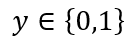
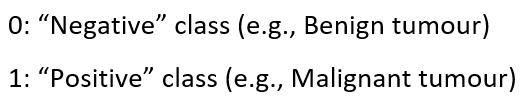
Classification problems can be explained based on the Breast Cancer dataset where there are two types of tumors (Benign and Malignant). It can be represented as:

where

This is a classification problem with 2 classes, 0 & 1. Generally, the classification problems have multiple classes say, 0,1,2 and 3.

Dataset:

The link to the Breast cancer dataset used in this article is given below:

Breast Cancer Wisconsin (Diagnostic) Data Set

Predict whether the cancer is benign or malignant

www.kaggle.com

1. Let’s import the dataset to a pandas dataframe:

import pandas as pd
read_df = pd.read_csv('breast_cancer.csv')
df = read_df.copy()

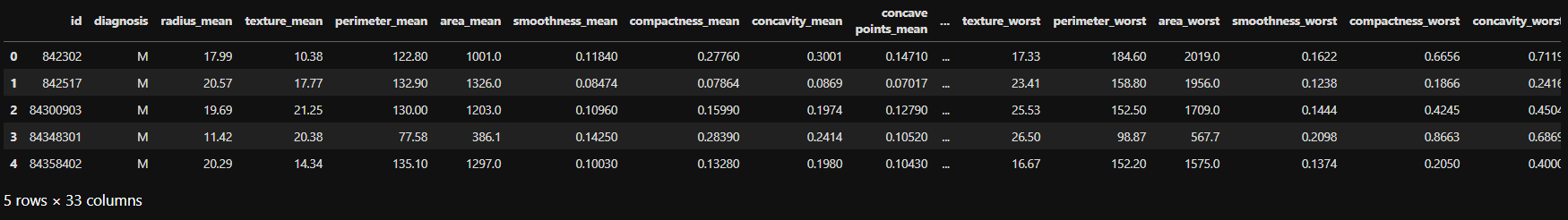
2. The following dataframe is obtained:

df.head()

 ![Image for post](https://miro.medium.com/max/1750/1*PPyiGgocvjHbgIcs9yTWTA.png)

df.info()

Data analysis:

Let us plot the mean area of the clump and its classification and see if we can find a relation between them.

import matplotlib.pyplot as plt
import seaborn as sns
from sklearn import preprocessing
label_encoder = preprocessing.LabelEncoder()
df.diagnosis = label_encoder.fit_transform(df.diagnosis)
sns.set(style = 'whitegrid')
sns.lmplot(x = 'area_mean', y = 'diagnosis', data = df, height = 10, aspect = 1.5, y_jitter = 0.1)

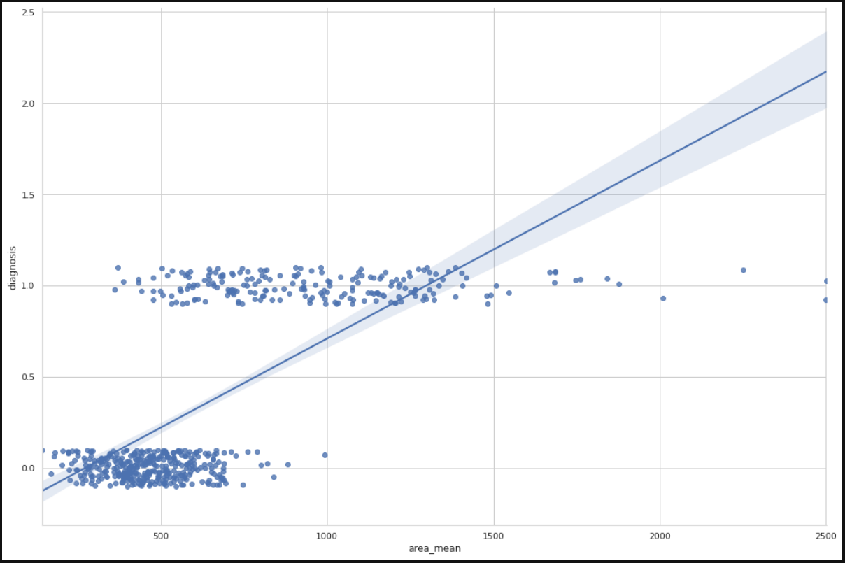
We can infer from the plot that most of the tumors having an area less than 500 are benign(represented by zero) and those having area more than 1000 are malignant(represented by 1). The tumors having a mean area between 500 to 1000 are both benign and malignant, therefore show that the classification depends on more factors other than mean area. A linear regression line is also plotted for further analysis.

#machine-learning #logistic-regression #regression #data-sceince #classification #deep learning