Data Preprocessing in Python

In this post I am going to walk through the implementation of Data Preprocessing methods using Python.

Data Preprocessing refers to the steps applied to make data more suitable for data mining. The steps used for Data Preprocessing usually fall into two categories:

1. selecting data objects and attributes for the analysis.
2. creating/changing the attributes.

In this post I am going to walk through the implementation of Data Preprocessing methods using Python. I will cover the following, one at a time:

1. Importing the libraries
2. Importing the Dataset
3. Handling of Missing Data
4. Handling of Categorical Data
5. Splitting the dataset into training and testing datasets
6. Feature Scaling

For this Data Preprocessing script, I am going to use Anaconda Navigator and specifically Spyder to write the following code. If Spyder is not already installed when you open up Anaconda Navigator for the first time, then you can easily install it using the user interface.

If you have not code in Python beforehand, I would recommend you to learn some basics of Python and then start here. But, if you have any idea of how to read Python code, then you are good to go. Getting on with our script, we will start with the first step.

Importing the libraries

# libraries

import numpy as np # used for handling numbers
import pandas as pd # used for handling the dataset
from sklearn.impute import SimpleImputer # used for handling missing data
from sklearn.preprocessing import LabelEncoder, OneHotEncoder # used for encoding categorical data
from sklearn.model_selection import train_test_split # used for splitting training and testing data
from sklearn.preprocessing import StandardScaler # used for feature scaling

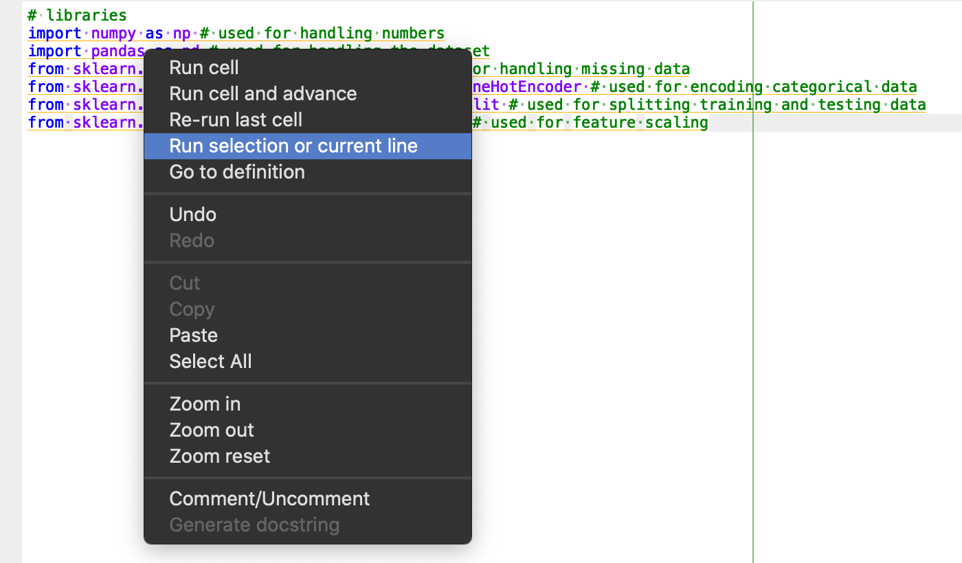
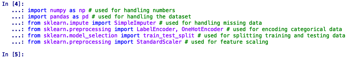
If you select and run the above code in Spyder, you should see a similar output in your IPython console.

If you see any import errors, try to install those packages explicitly using pip command as follows.

pip install <package-name>

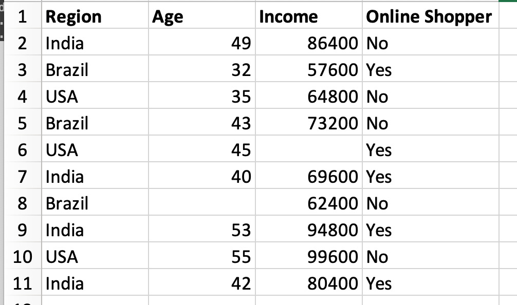
Importing the Dataset

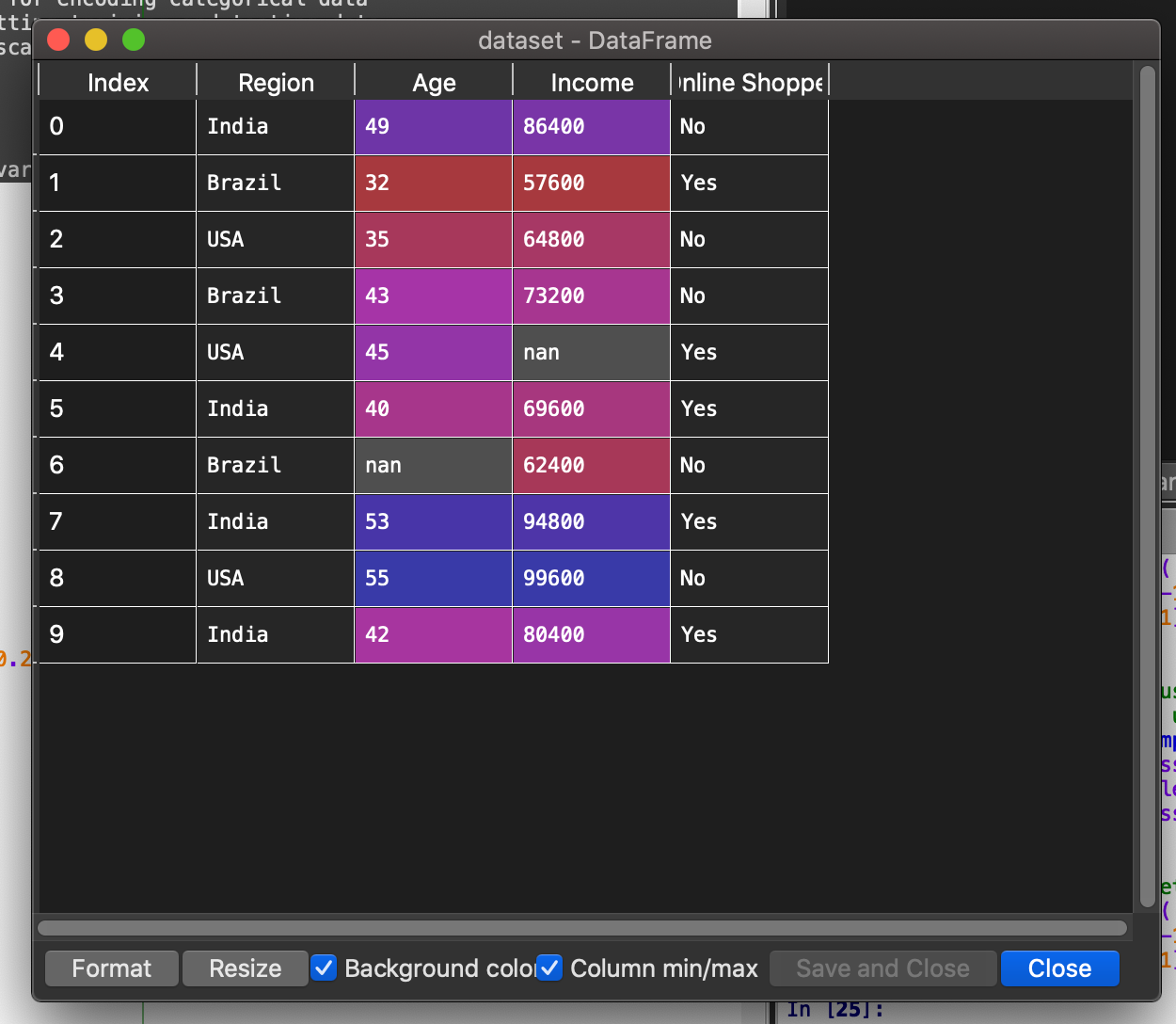
First of all, let us have a look at the dataset we are going to use for this particular example.

In order to import this dataset into our script, we are apparently going to use pandas as follows.

dataset = pd.read_csv('Data.csv') # to import the dataset into a 
variable

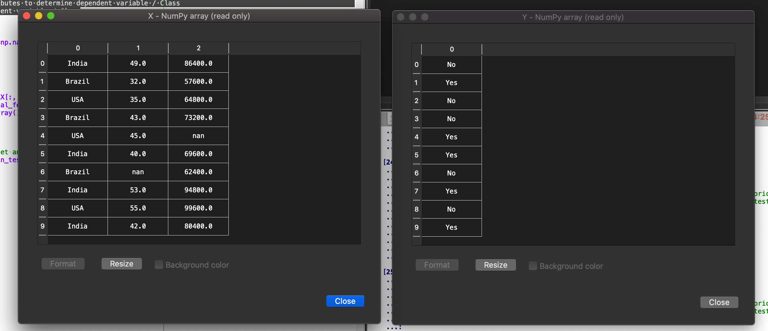
# Splitting the attributes into independent and dependent attributes
X = dataset.iloc[:, :-1].values # attributes to determine dependent variable / Class
Y = dataset.iloc[:, -1].values # dependent variable / Class

When you run this code section, you should not see any errors, if you do make sure the script and the *Data.csv *are in the same folder. When successfully executed, you can move to variable explorer in the Spyder UI and you will see the following three variables.

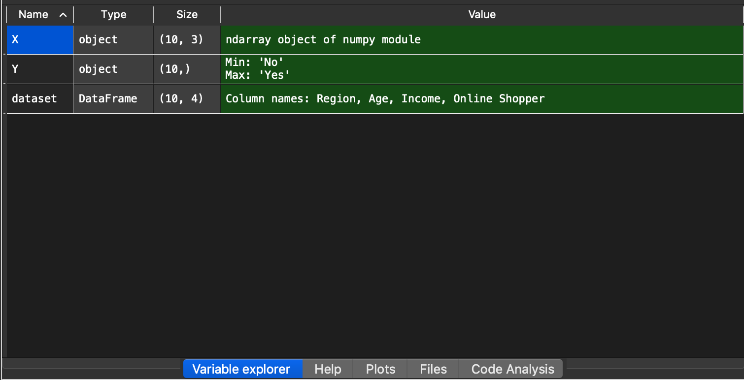
When you double click on each of these variables, you should see something similar.

If you face any errors in order to see these data variables, try to upgrade Spyder to Spyder version 4.

Handling of Missing Data

Well the first idea is to remove the lines in the observations where there is some missing data. But that can be quite dangerous because imagine this data set contains crucial information. It would be quite dangerous to remove an observation. So we need to figure out a better idea to handle this problem. And another idea that’s actually the most common idea to handle missing data is to take the mean of the columns.

If you noticed in our dataset, we have two values missing, one for age column in 7th data row and for Income column in 5th data row. Missing values should be handled during the data analysis. So, we do that as follows.

# handling the missing data and replace missing values with nan from numpy and replace with mean of all the other values
imputer = SimpleImputer(missing_values=np.nan, strategy='mean') imputer = imputer.fit(X[:, 1:])
X[:, 1:] = imputer.transform(X[:, 1:])

After execution of this code, the independent variable *X *will transform into the following.

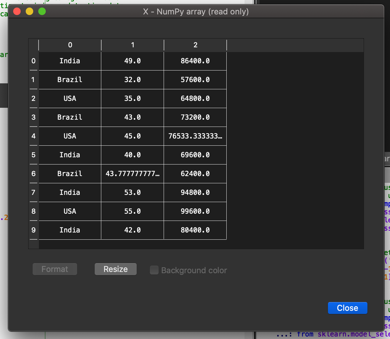
Here you can see, that the missing values have been replaced by the average values of the respective columns.

Handling of Categorical Data

In this dataset we can see that we have two categorical variables. We have the Region variable and the Online Shopper variable. These two variables are categorical variables because simply they contain categories. The Region contains three categories. It’s India, USA & Brazil* *and the online shopper variable contains two categories. Yes and No that’s why they’re called categorical variables.

You can guess that since machine learning models are based on mathematical equations you can intuitively understand that it would cause some problem if we keep the text here in the categorical variables in the equations because we would only want numbers in the equations. So that’s why we need to encode the categorical variables. That is to encode the text that we have here into numbers. To do this we use the following code snippet.

# encode categorical data
from sklearn.preprocessing import LabelEncoder, OneHotEncoder
labelencoder_X = LabelEncoder()
X[:, 0] = labelencoder_X.fit_transform(X[:, 0])
onehotencoder = OneHotEncoder(categorical_features=[0])
X = onehotencoder.fit_transform(X).toarray()
labelencoder_Y = LabelEncoder()
Y = labelencoder_Y.fit_transform(Y)

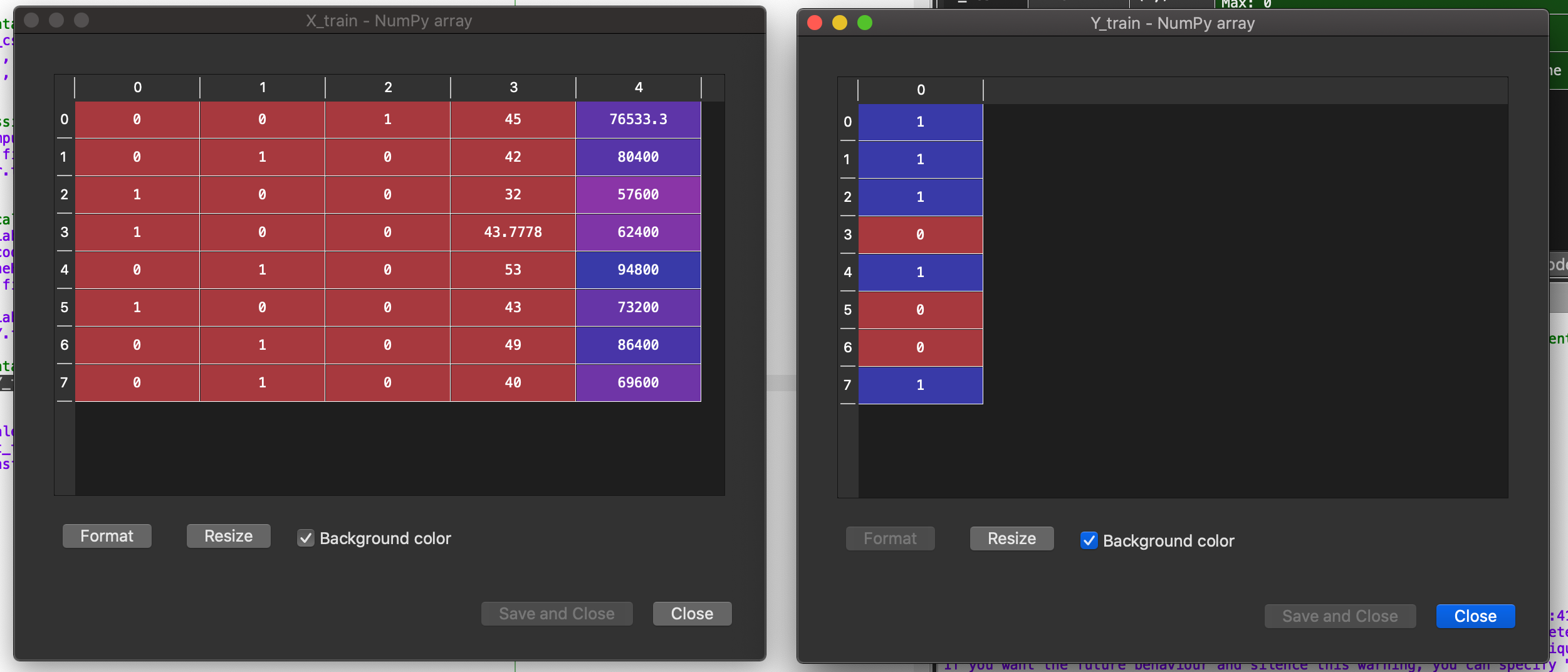
After execution of this code, the independent variable *X *and dependent variable *Y *will transform into the following

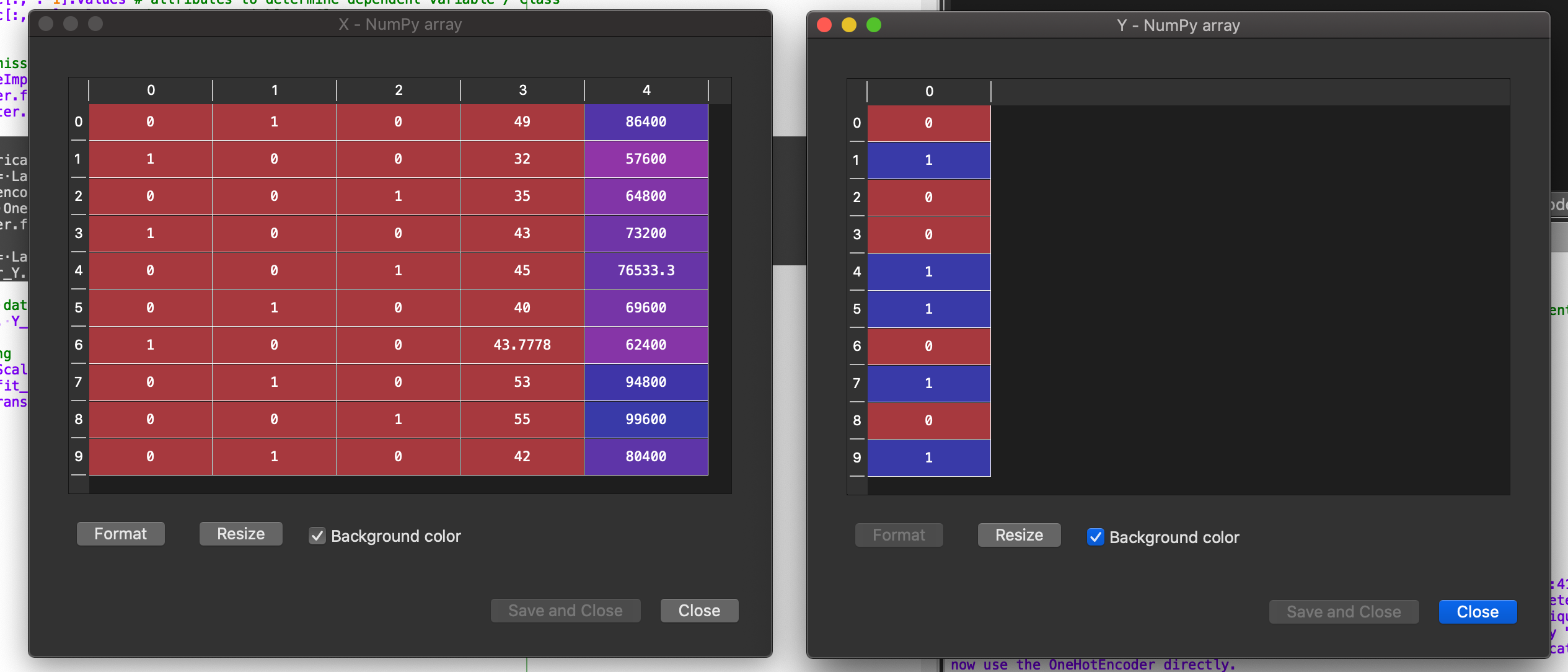
Here, you can see that the Region variable is now made up of a 3 bit binary variable. The left most bit represents ***India, ***2nd bit represents ***Brazil ***and the last bit represents ***USA. ***If the bit is **1 then it represents data for that country otherwise not. For Online Shopper variable, 1 represents Yes and 0represents No.

Splitting the dataset into training and testing datasets

Any machine learning algorithm needs to be tested for accuracy. In order to do that, we divide our data set into two parts: **training set **and **testing set.**As the name itself suggests, we use the training set to make the algorithm learn the behaviours present in the data and check the correctness of the algorithm by testing on testing set. In Python, we do that as follows:

# splitting the dataset into training set and test set
X_train, X_test, Y_train, Y_test = train_test_split(X, Y, test_size=0.2, random_state=0)

Here, we are taking training set to be 80% of the original data set and testing set to be 20% of the original data set. This is usually the ratio in which they are split. But, you can come across sometimes to a 70–30% or 75–25% ratio split. But, you don’t want to split it 50–50%. This can lead to ***Model Overfitting. ***This topic is too huge to be covered in the same post. I will cover it in some future post. For now, we are going to split it in 80–20% ratio.

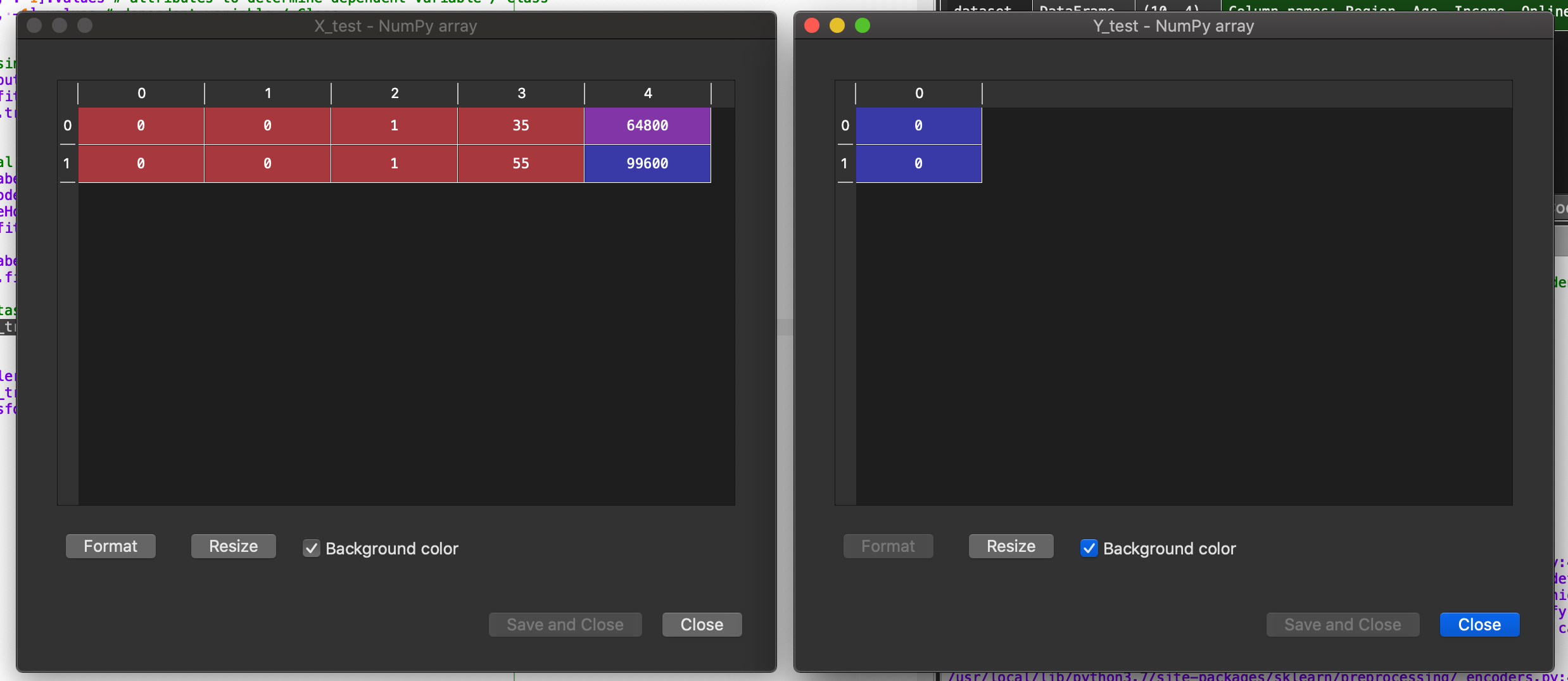
After split, our training set and testing set look like this.

Feature Scaling

As you can see we have these two columns age and income that contains numerical numbers. You notice that the variables are not on the same scale because the age are going from 32 to 55 and the salaries going from 57.6 K to like 99.6 K.

So because this age variable in the salary variable don’t have the same scale. This will cause some issues in your machinery models. And why is that. It’s because your machine models a lot of machinery models are based on what is called the Euclidean distance.

We use feature scaling to convert different scales to a standard scale to make it easier for Machine Learning algorithms. We do this in Python as follows:

# feature scaling

sc_X = StandardScaler()
X_train = sc_X.fit_transform(X_train)
X_test = sc_X.transform(X_test)

After the execution of this code, our training independent variable *X *and our testing independent variable *X and *look like this.

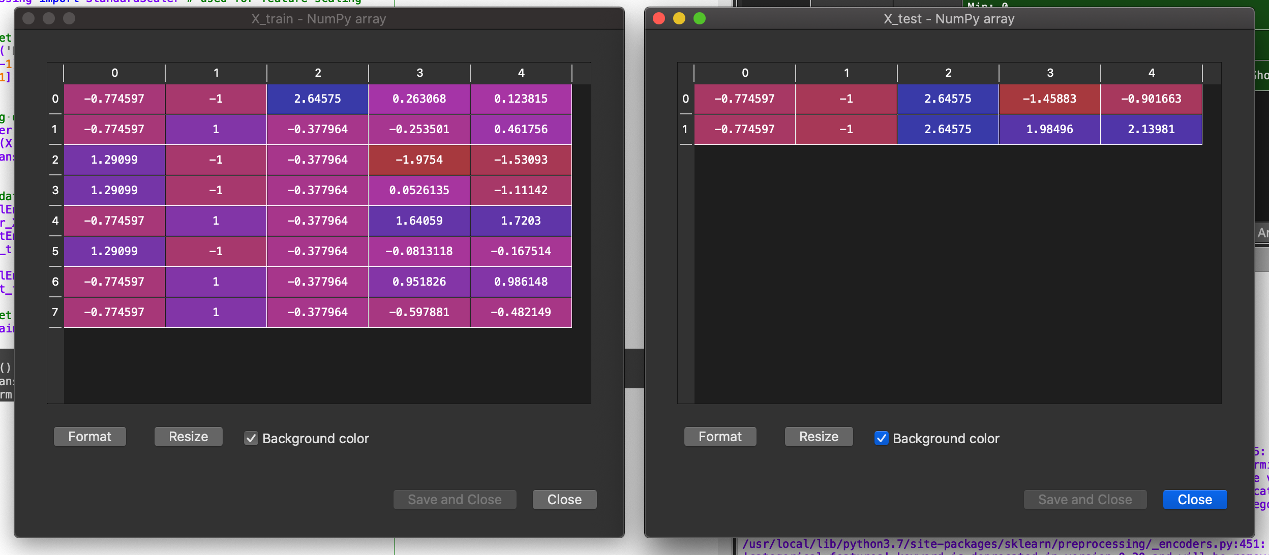
This data is now ready to be fed to a Machine Learning Algorithm.This concludes this post on Data Preprocessing in Python.

#machine-learning #python #data-science