在先前的文章中已經教了比正規方程更好用的梯度遞減。但是，在什麼樣的情況下，原本的梯度遞減公式還是會不適用呢？

給定Kaggle資料集艾姆斯房價資料為例，若以其中的 GrLivArea 作為特徵矩陣來預測目標向量 Saleprice。

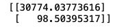
使用 Scikit-Learn 的 Linear Regression 預測器找出 𝑤:

import pandas as pd
import numpy as np
from sklearn.model_selection import train_test_split
from sklearn.linear_model import LinearRegression

csv_url = "https://kaggle-getting-started.s3-ap-northeast-1.amazonaws.com/house-prices/train.csv"
housing = pd.read_csv(csv_url)
X = housing["GrLivArea"].values.reshape(-1, 1)
y = housing["SalePrice"].values
X_train, X_validation, y_train, y_validation = train_test_split(X, y, test_size=0.33, random_state=42)
lr = LinearRegression()
lr.fit(X_train, y_train)
w = lr.coef_.copy()
w = np.insert(w, 0, lr.intercept_).reshape(-1, 1)
print(w)

使用 Gradient Descent 找出 𝑤：

def get_mse(X, y, w):
    m = y.size
    y_hat = X.dot(w)
    y_reshaped = y.reshape(-1, 1)
    err = y_hat - y_reshaped
    se = err**2
    sse = se.sum()
    mse = sse / m
    return mse

def get_grad(X, y, w):
    m = y.size
    y_hat = X.dot(w)
    y_reshaped = y.reshape(-1, 1)
    err = y_hat - y_reshaped
    grad = (X.T.dot(err))*2/m
    return grad

def gradient_descent(X, y, epochs, learning_rate):
    n = X.shape[1]
    w = np.random.rand(n, 1)
    j_history = []
    w_0_history, w_1_history = [w[0, 0]], [w[1, 0]]
    n_prints = 20
    interval = epochs // n_prints
    for i in range(epochs):
        mse = get_mse(X, y, w)
        j_history.append(mse)
        grad = get_grad(X, y, w)
        w -= learning_rate*grad
        if i % interval == 0:
            w_0_history.append(w[0, 0])
            w_1_history.append(w[1, 0])
            print("{} iterations: w_0 = {}; w_1 = {}".format(i, w[0, 0], w[1, 0]))
    return w, w_0_history, w_1_history, j_history

from sklearn.preprocessing import PolynomialFeatures

poly = PolynomialFeatures(1)
X_poly = poly.fit_transform(X)
X_train, X_validation, y_train, y_validation = train_test_split(X_poly, y, test_size=0.33, random_state=42)
n_epochs = 300000
learning_rate = 1e-7
w, w_0_history, w_1_history, j_history = gradient_descent(X_train, y_train, n_epochs, learning_rate)

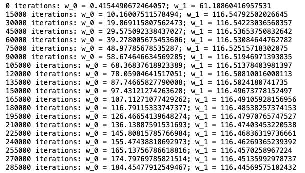
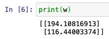
我們發現透過梯度遞減演算法找的w，w0的值(194)與正確解答(30774)還差了十萬八千里。我們試著作圖了解一下原因：

import matplotlib.pyplot as plt

def get_gd_plots(j_history, w_0_history, w_1_history, best_w_0, best_w_1):
    fig, axes = plt.subplots(1, 2, figsize=(12, 3))
    axes[0].plot(range(len(j_history)), j_history)
    axes[0].set_xlabel("Number of iterations")
    axes[0].set_ylabel("MSE")
    axes[0].set_title("MSE trend")
    axes[1].scatter(w_0_history, w_1_history, marker="+")
    axes[1].scatter(best_w_0, best_w_1, marker="x", s=200, color="red")
    axes[1].scatter(w_0_history[-1], w_1_history[-1], marker="x", s=200, color="green")
    axes[1].set_xlabel("$w_0$")
    axes[1].set_ylabel("$w_1$")
    axes[1].set_title("How does $w_0$ and $w_1$ converge")
    #axes[1].set_ylim(0, 15)
    plt.show()
    
get_gd_plots(j_history, w_0_history, w_1_history, 30774, 98.5)

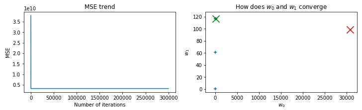
由於在一開始迭代時，MSE就已經是最小了，所以w0才會每次只動一點點，造成w0無法抵達最佳解的值。

#python #machine-learning #機器學習